Example of Generalized Regression

The data in the Diabetes.jmp sample data table consist of measurements on 442 diabetics. The response of interest is Y, disease progression measured one year after a baseline measure was taken. Ten variables thought to be related to disease progression are also measured at baseline. This example shows how to develop a predictive model using generalized regression techniques.

1.	Select Help > Sample Data Library and open Diabetes.jmp.

2.	Select Analyze > Fit Model.

3.	Select Y from the Select Columns list and click Y.

4.	Select Age through Glucose and click Macros > Factorial to degree.

This adds all terms up to degree 2 (the default in the Degree box) to the model.

5.	Select Validation from the Select Columns list and click Validation.

6.	From the Personality list, select Generalized Regression.

7.	Click Run.

The Generalized Regression Model Launch control panel appears. Note that the default estimation method is the adaptive Lasso.

Because you specified a validation column in the Fit Model window, the Validation Method is set to Validation Column.

Click Go.

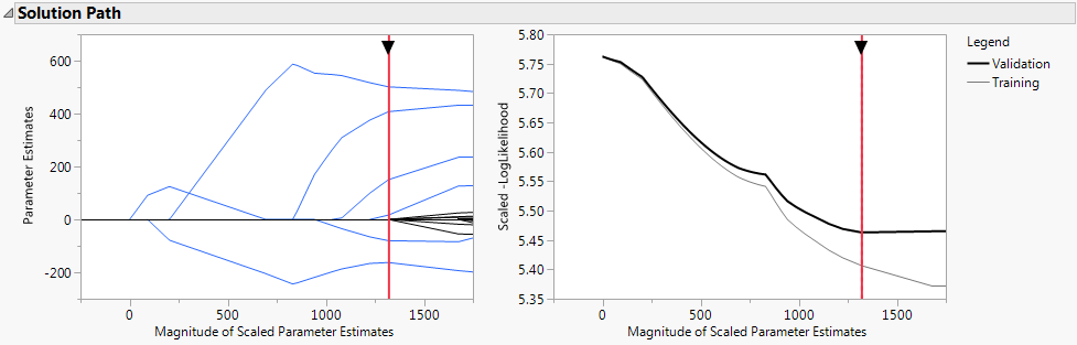
The Solution Path report (Solution Path Plot) shows plots of the parameter estimates and scaled negative log likelihood. The shrinkage increases as the Magnitude of Scaled Parameter Estimates decreases. The estimates at the far right of the plot are the maximum likelihood estimates. A vertical red line indicates those parameter values selected by the validation criterion, in this case, the holdback sample defined by the column Validation.

Solution Path Plot

9.	Select the option Select Nonzero Terms from the Adaptive Lasso with Validation Column Validation report’s red triangle menu.

This option highlights the nonzero terms in the Parameter Estimates for Original Data report (Portion of Parameter Estimates for Original Predictors Report) and their paths in the Solution Path plot. The corresponding columns in the data table are also selected. Note that only 6 of the 55 parameter estimates are nonzero. Also note that the scale parameter for the normal distribution (sigma) is estimated and shown in the last line of the Parameter Estimates for Original Data report.

Portion of Parameter Estimates for Original Predictors Report

To save the prediction formula, select Save Columns > Save Prediction Formula from the red triangle menu for the Adaptive Lasso with Validation Column Validation report.

Launch the Generalized Regression Personality

Launch the Generalized Regression personality by selecting Analyze > Fit Model, entering one or more columns for Y, and selecting Generalized Regression from the Personality menu (Fit Model Launch Window with Generalized Regression Selected).

Fit Model Launch Window with Generalized Regression Selected

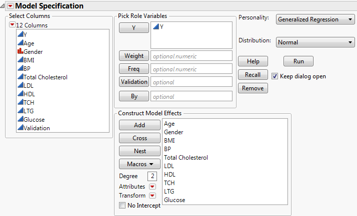
For details about aspects of the Fit Model window that are common to all personalities, see the Model Specification section. Details specific to the Generalized Regression personality are presented here.

If your model effects have missing values, you can treat these missing values as informative categories. Select the Informative Missing option from the Model Specification window’s red triangle menu.

To specify a model without an intercept term, select the No Intercept option in the Construct Model Effects panel of the Fit Model window. Categorical effects are not supported by the No Intercept option. When the No Intercept option is selected, Maximum Likelihood and Forward Selection are the only estimation methods available in the Model Launch specification. When the No Intercept option is selected, the predictors are not centered and scaled.

Distribution

When you select Generalized Regression from the Personality menu, the Distribution option appears. Here you can specify a distribution for Y. The abbreviation ZI means zero-inflated. The distributions are separated into three categories based on their response: continuous, discrete, and zero-inflated. The options are described below.

Continuous

Normal

Y has a normal distribution with mean μ and standard deviation σ. The normal distribution is symmetric and with a large enough sample size, can approximate a large variety of other distributions using the Central Limit Theorem. The link function for μ is the identity. That is, the mean of Y is expressed as a linear model. In estimating the model parameters, the scale parameter σ is profiled out. It is then replaced by its maximum likelihood estimate (MLE). (Note that the MLE is not the typical unbiased estimator for σ.) See Statistical Details for Distributions.

Cauchy

Y has a Cauchy distribution with location parameter μ and scale parameter σ. The Cauchy distribution has an undefined mean and standard deviation. The median and mode are both μ. Most data do not inherently follow a Cauchy distribution, but it is useful for conducting a robust regression on data that contain a large proportion of outliers (up to 50%). The link function for μ and σ is the identity. See Statistical Details for Distributions.

Exponential

Y has an exponential distribution with mean parameter μ. The exponential distribution is right-skewed and is often used to model lifetimes or the time between successive events. The link function for μ is the logarithm. See Statistical Details for Distributions.

Gamma

Y has a gamma distribution with mean parameter μ and dispersion parameter σ. The gamma is a flexible distribution and contains a family of other widely used distributions. For example, the exponential distribution is a special case of the gamma distribution where σ = μ. The Weibull and chi squared distributions can also be derived from the gamma distribution. The link function for μ is the logarithm. See Statistical Details for Distributions.

Beta

Y has a beta distribution with mean parameter μ and dispersion parameter σ. The response for the beta is between 0 and 1 (not inclusive) and is often used to model proportions or rates. The link function for μ is the logit. See Statistical Details for Distributions.

Quantile Regression

Quantile regression models a specified conditional quantile of the response. No assumption is made about the form of the underlying distribution. When you select Quantile Regression, a Quantile box appears beneath the Distribution menu. Specify the desired quantile.

If you specify 0.5 (the default) for the Quantile on the Model Dialog window, quantile regression models the conditional median of the response. Quantile regression is particularly useful when the rate of change in the conditional quantile, expressed by the regression coefficients, depends on the quantile. An advantage of quantile regression over least squares regression is its flexibility for modeling data with heterogeneous conditional distributions.

Quantile Regression is fit by minimizing an objective function using an iterative approach. For more information about quantile regression, see Koenker and Hallock (2001), Portnoy and Koenker (1997), and Sánchez et al. (2013).

When you choose Quantile Regression, Maximum Likelihood is the only available Estimation Method, and None is the only available Validation Method.

Note: If a quantile regression fit is time intensive, a progress bar appears. The progress bar shows the relative change in the objective function. When you click Accept Current Estimates, the calculation stops and the reported parameter estimates correspond to the best model fit at that point.

Discrete

Binomial

Y has a binomial distribution with parameters p and n. The response, Y, indicates the total number of successes in n independent trials with a fixed probability, p, for all trials. This distribution allows for the use of a sample size column. If no column is listed, it is assumed that the sample size is one. The link function for p is the logit. When you select Binomial as the Distribution, the response variable must be specified in one of the following ways. See Statistical Details for Distributions.

‒	Unsummarized: If your data are not summarized as frequencies of events, specify a single binary column as the response.

‒	Summarized with Freq column: If your data are summarized as frequencies of successes and failures, specify a single binary column as the response. This column can have any modeling type. Assign the frequency column to the Freq role.

‒	Summarized with sample size column entered as second Y: If your data are summarized as frequencies of events (successes) and trials, specify two continuous columns as Y in this order: the count of the number of successes, and the count of the number of trials.

Beta Binomial

Y has a beta binomial distribution with the probability of success, p, the number of trails, n, and overdispersion parameter, δ. This distribution is an overdispersed version of the binomial distribution.

Run demoBetaBinomial.jsl in the JMP Samples/Scripts folder to compare a beta binomial distribution with dispersion parameter δ to a binomial distribution with parameters p and n = 20.

The beta binomial distribution requires a sample size greater than one for each observation. Thus, the user must specify a sample size column. To insert a sample size column, specify two continuous columns as Y in this order: the count of the number of successes, and the count of the number of trials. The link function for p is the logit. See Statistical Details for Distributions.

Poisson

Y has a Poisson distribution with mean λ. The Poisson distribution typically models the number of events in a given interval and is often expressed as count data. The link function for λ is the logarithm. Poisson regression is permitted even if Y assumes non-integer values. See Statistical Details for Distributions.

Negative Binomial

Y has a negative binomial distribution with mean μ and dispersion parameter σ. The negative binomial distribution typically models the number of successes before a specified number of failures. The negative binomial distribution is also equivalent to the Gamma Poisson distribution under certain conditions. For more details about the connection between negative binomial and Gamma Poisson, see the Distributions chapter in the Basic Analysis book.

Run demoGammaPoisson.jsl in the JMP Samples/Scripts folder to compare a Gamma Poisson distribution with mean λ and dispersion parameter σ to a Poisson distribution with mean λ.

The link function for μ is the logarithm. Negative binomial regression is permitted even if Y assumes non-integer values. See Statistical Details for Distributions.

Zero-Inflated

ZI Binomial

Y has a zero-inflated binomial distribution with parameters p, n, and zero-inflation parameter π. The response, Y, indicates the total number of successes in n independent trials with a fixed probability, p, for all trials. This distribution allows for the use of a sample size column. If no column is listed, it is assumed that the sample size is one. The link function for p is the logit. See Statistical Details for Distributions.

ZI Beta Binomial

Y has a beta binomial distribution with the probability of success, p, the number of trails, n, overdispersion parameter, δ, and zero-inflation parameter π. This distribution is an overdispersed version of the ZI binomial distribution. The ZI beta binomial distribution requires a sample size greater than one for each observation. Thus, the user must specify a sample size column. To insert a sample size column, specify two continuous columns as Y in this order: the count of the number of successes, and the count of the number of trials. The link function for p is the logit. See Statistical Details for Distributions.

ZI Poisson

Y has a zero-inflated Poisson distribution with mean parameter λ and zero-inflation parameter π. The parameter λ is the conditional mean based on the observations coming from the Poisson distribution and not the inflating zeros. The link function for λ is the logarithm. ZI Poisson regression is permitted even if Y assumes no observed zeros or non-integer values. See Statistical Details for Distributions.

ZI Negative Binomial

Y has a zero-inflated negative binomial with location parameter μ, dispersion parameter σ, and zero-inflation parameter π. The parameter μ is the conditional mean based on the observations coming from the negative binomial distribution and not the inflating zeros. The link function for μ is the logarithm. ZI negative binomial regression is permitted even if Y assumes no observed zeros or non-integer values. See Statistical Details for Distributions.

ZI Gamma

Y has a zero-inflated gamma distribution with mean parameter μ and zero-inflation parameter π. Many times, we might believe that our nonzero responses are gamma distributed. This is true for insurance claims: claim values are approximately gamma distributed but there are also zeros in the data for policies that do not have any claims. The zero-inflated gamma could handle such data directly without having to split the data into zero and nonzero responses. The parameter μ is the conditional mean based on observations coming from the gamma distribution and not the inflating zeros. The link function for μ is the logarithm. See Statistical Details for Distributions.

Requirements for Y for Distributions gives the Data Types, Modeling Types, and other requirements for Y variables assigned the various distributions.

Requirements for Y for Distributions
Distribution	Data Type	Modeling Type	Other
Normal	Numeric	Continuous
Cauchy	Numeric	Continuous
Exponential	Numeric	Continuous	Positive
Gamma	Numeric	Continuous	Positive
Beta	Numeric	Continuous	Between 0 and 1
Quantile Regression	Numeric	Continuous
Binomial, unsummarized	Any	Any	Binary
Binomial, summarized with Freq column	Any	Any	Binary
Binomial, summarized with count column entered as second Y	Numeric	Continuous	Nonnegative
Beta Binomial	Numeric	Continuous	Nonnegative
Poisson	Numeric	Any	Nonnegative
Negative Binomial	Numeric	Any	Nonnegative
Zero-Inflated Binomial	Numeric	Any	Nonnegative
Zero-Inflated Beta Binomial	Numeric	Any	Nonnegative
Zero-Inflated Poisson	Numeric	Any	Nonnegative
Zero-Inflated Negative Binomial	Numeric	Any	Nonnegative
Zero-Inflated Gamma	Numeric	Continuous	Nonnegative

Details on how these distributions are parameterized are given in Statistical Details for Distributions. Distributions, Parameters, and Link Functions summarizes the details.

Distributions, Parameters, and Link Functions
Distribution	Parameters	Mean Model Link Function
Normal	μ, σ
Cauchy	μ, σ
Exponential	μ
Gamma	μ, σ
Beta	μ
Binomial	n, p
Beta Binomial	n, p, δ
Poisson	λ
Negative Binomial	μ, σ
Zero-Inflated Binomial	n, p, π (zero-inflation)
Zero-Inflated Beta Binomial	n, p, δ, π (zero-inflation)
Zero-Inflated Poisson	λ, π (zero-inflation)
Zero-Inflated Negative Binomial	μ, σ, π (zero-inflation)
Zero-Inflated Gamma	μ, σ, π (zero-inflation)

After selecting an appropriate Distribution, click Run. The Generalized Regression Model Launch panel opens.

Model Launch Window

The Model Launch window provides options for the following:

•	Estimation Method Options

•	Advanced Controls

•	Validation Method Options

•	Early Stopping

•

Estimation Method Options

Ridge, the Lasso, and the Elastic Net are penalized regression techniques. They shrink the size of regression coefficients, thus biasing them, in order to improve predictive ability. By default, Generalized Regression fits adaptive versions of the Lasso and Elastic Net.

Note: When your data are highly collinear, the adaptive versions of Lasso and Elastic Net might not provide good solutions. This is because the adaptive versions presume that the MLE provides a good estimate. Uncheck the Adaptive option in such cases.

Two types of penalties are used in these techniques:

•	the l1 penalty, which penalizes the sum of the absolute values of the regression coefficients

•	the l2 penalty, which penalizes the sum of the squares of the regression coefficients

The following methods are available for model fitting:

Maximum Likelihood

Computes maximum likelihood estimates (MLEs) for model parameters. No penalty is imposed. Maximum Likelihood is the only estimation method available for Quantile Regression.

Forward Selection

Computes effect estimates using forward stepwise regression. The model chosen provides the best solution relative to the selected Validation Method.

Ridge

Computes parameter estimates using ridge regression. This technique applies an l2 penalty. See Statistical Details for Estimation Methods.

Lasso

Computes parameter estimates by applying an l1 penalty. Due to the l1 penalty, some coefficients can be estimated as zero. Thus, variable selection is performed as part of the fitting procedure. In the ordinary Lasso, all coefficients are equally penalized. See Statistical Details for Estimation Methods.

Adaptive Lasso

Computes parameter estimates by penalizing a weighted sum of the absolute values of the regression coefficients. The weights in the l1 penalty are determined by the data in such as way as to guarantee the oracle property (Zou, 2006). This option uses the MLEs to weight the l1 penalty. MLEs cannot be computed when the number of predictors exceeds the number of observations or when there are strict linear dependencies among the predictors. If MLEs for the regression parameters cannot be computed, a generalized inverse solution or a ridge solution is used for the l1 penalty weights. See Statistical Details for Estimation Methods.

Elastic Net

Computes parameter estimates by applying both an l1 penalty and an l2 penalty. The l1 penalty ensures that variable selection is performed. The l2 penalty improves predictive ability by shrinking the coefficients as ridge does. See Statistical Details for Estimation Methods.

Adaptive Elastic Net

Computes parameter estimates using an adaptive l1 penalty as well as an l2 penalty. This option uses the MLEs to weight the l1 penalty. MLEs cannot be computed when the number of predictors exceeds the number of observations or when there are strict linear dependencies among the predictors. If MLEs for the regression parameters cannot be computed, a generalized inverse solution or a ridge solution is used for the l1 penalty weights. You can set a value for the Elastic Net Alpha in the Advanced Controls panel. See Statistical Details for Estimation Methods.

Note: If you select an Elastic Net fit and set the Elastic Net Alpha to missing, the algorithm computes the Lasso, Elastic Net, and Ridge fits, in that order. If a fit is time intensive, a progress bar appears. When you click Accept Current Estimates, the calculation stops and the reported parameter estimates correspond to the best model fit at that point. The progress bar indicates when the algorithm is fitting Lasso, Elastic Net, and Ridge. You can use this information to decide when to click Accept Current Estimates.

Discussion of Estimation Methods

The Maximum Likelihood option gives you a way to construct classical models for the response distributions supported by the Generalized Regression personality. In addition, a model based on maximum likelihood can serve as a baseline for model comparison.

Ridge regression is a biased regression technique that does not result in zero parameter estimates. It is useful when you want to retain all predictors in your model.

The Lasso and the adaptive Lasso options generally choose parsimonious models when predictors are highly correlated. These techniques tend to select only one of a group of correlated predictors. High-dimensional data tend to have highly correlated predictors. For this type of data, the Elastic Net might be a better choice than the Lasso.

The Elastic Net tends to provide better prediction accuracy than the Lasso when predictors are highly correlated. (In fact, both Ridge and the Lasso are special cases of the Elastic Net.) In terms of predictive ability, the adaptive Elastic Net often outperforms both the Elastic Net and the adaptive Lasso. The Elastic Net has the ability to select groups of correlated predictors and to assign appropriate parameter estimates to the predictors involved.

Advanced Controls

Use the Advanced Controls options to adjust various aspects of the model fitting process. A number of controls relate to the grid for the tuning parameter.

Tuning Parameter

The solution paths for the Lasso and Ridge Estimation Methods depend on a single tuning parameter. The solution path for the Elastic Net depends on a tuning parameter for the penalty on the likelihood as well as the Elastic Net Alpha. The penalty on the likelihood for the Elastic Net is a weighted sum of the penalties associated with the Lasso and Ridge Estimation Methods. The Elastic Net Alpha determines the weights of these two penalties. See Statistical Details for Estimation Methods and Statistical Details for Advanced Controls.

When the tuning parameter is zero, the solution is unpenalized and maximum likelihood estimates are obtained. As the tuning parameter increases, the penalty increases.

The solution is the set of parameter estimates that minimizes the penalized likelihood relative to the selected validation method. The current solution is designated by the red vertical line in the Solution Path plots.

Note: The value of the tuning parameter increases as the Magnitude of Scaled Parameter Estimates in the Solution Path plot decreases. Estimates close to the MLE are associated with large magnitudes and estimates that are heavily penalized are associated with small magnitudes.

It is important to be mindful of the following:

•	When the tuning parameter is too small, the data are typically overfit and result in models with high variance.

•	When the tuning parameter is too large, the data are typically underfit.

The Tuning Parameter Grid

To obtain a solution, the tuning parameter is increased over a fine grid.

•	For the Lasso, Elastic Net with Elastic Net Alpha specified, and Ridge, the value of the tuning parameter that gives the solution is the one that provides the best fit over the grid of tuning parameters.

Note: Elastic Net Alpha is set to 0.9 by default.

•

If you do not set a value for the Elastic Net Alpha, the value of alpha is also increased over a fine grid. For a fixed value of the tuning parameter, alpha is varied until ten consecutive values of alpha fail to improve upon the best fit as determined by the validation method. This process is repeated for the entire grid of tuning parameter values. The final values of the tuning parameter and alpha are the values that provide the best fit over the grid of tuning parameters.

The grid of tuning parameter values ranges from zero, in most cases, to the smallest value for which all of the non-intercept terms are zero. Define the smallest value of the tuning parameter for which all non-intercept terms are zero to be its upper bound. The lower bound for the tuning parameter is zero except in the following two cases where it is set to 0.01:

•	If the design matrix is singular, the maximum likelihood estimates cannot be computed. The lower bound of 0.01 allows estimates close to the MLEs to be computed.

•	If the selected distribution is binomial, the lower bound of 0.01 helps prevent separation.

Advanced Control Options

Enforce effect heredity

Requires lower-order effects to enter the model before their related higher order effects. In most cases, this means that X2 is not in the model unless X is in the model. For estimation methods other than Forward Selection, however, it is possible for X2 to enter the model and X to leave the model in the same step. If the data table contains a DOE script, this option is enabled, but it is off by default.

Elastic Net Alpha

Sets the α parameter for the Elastic Net. This α parameter determines the mix of the l1 and l2 penalty tuning parameters in estimating the Elastic Net coefficients. The default value is α = 0.9, which sets the coefficient on the l1 penalty to 0.9 and the coefficient on the l2 penalty to 0.1. This option is available only when Elastic Net is selected as the Estimation Method. See Statistical Details for Estimation Methods.

Number of Grid Points

Specifies the number of grid points between the lower and upper bounds for the tuning parameter. At each grid point value, parameter estimates for that value of the tuning parameter are obtained. The default value is 150 grid points.

Minimum Penalty Fraction

Indicates the minimum value for the ratio of the lower bound of the tuning parameter to its upper bound. When the lower bound for the tuning parameter is 0, the solution provides the MLE. In cases where you do not want to include the MLE or solutions very close to it, you can set the Minimum Penalty Fraction to a nonzero value.

Grid Scale

Provides options for choosing the distribution of the grid scale. You can choose between a linear, square root, or log scale. Grid points equal in number to the specified Number of Grid Points are distributed according to the selected scale between the lower and upper bounds of the tuning parameter. See Statistical Details for Advanced Controls.

Force Terms

Enables you to select which terms, if any, you want to force into the model. The terms that are forced into the model are not included in the penalty.

Validation Method Options

The following methods are available for validation of the model fit.

Note: The only Validation Method allowed for Quantile Regression and for the Maximum Likelihood estimation method is None.

KFold

For each value of the tuning parameter, the following steps are conducted:

‒	The observations are partitioned into k subsets, or folds.

‒	In turn, each fold is used as a validation set. A model is fit to the observations not in the fold. The LogLikelihood based on that model is calculated for the observations in the fold, providing a validation LogLikelihood.

‒	The mean of the validation LogLikelihoods for the k folds is calculated. This value serves as a validation LogLikelihood for the value of the tuning parameter.

The value of the tuning parameter that has the maximum validation LogLikelihood is used to construct the final solution. To obtain the final model, all k models derived for the optimal value of the tuning parameter are fit to the entire data set. Of these, the model that has the highest LogLikelihood is selected as the final model. The training set used for that final model is designated as the Training set and the holdout fold for that model is the Validation set. These are the Training and Validations sets used in plots and results in the report for the final solution.

Holdback

Randomly selects the specified proportion of the data for a validation set, and uses the other portion of the data to fit the model. The final solution is the one that minimizes -LogLikelihood for the validation set. This method is useful for large data sets.

Leave-One-Out

Performs leave-one-out cross validation. This is equivalent to KFold, with the number of folds equal to the number of rows. This option should not be used on moderate or large data sets. It can require long processing time for even a moderate number of observations.

BIC

Minimizes the Bayesian Information Criterion (BIC) over the solution path. For more details, see Likelihood, AICc, and BIC in Statistical Details.

AICc

Minimizes the corrected Akaike Information Criterion (AICc) over the solution path. AICc is the default setting for Validation Method. For more details, see Likelihood, AICc, and BIC in Statistical Details.

Note: The AICc is not defined when the number of parameters approaches or exceeds the sample size.

None

Does not use validation. Only available for the Maximum Likelihood Estimation Method and Quantile Regression.

Validation Column

Uses the column specified in the Fit Model window as having the Validation role. The final solution is the one that minimizes -LogLikelihood for the validation set. This option is not available for Quantile Regression.

Early Stopping

Early Stopping adds an early stopping rule:

•	For Forward Selection, the algorithm terminates when 10 consecutive steps of adding variables to the model fail to improve upon the validation measure. The solution is the model at the step that precedes the 10 consecutive steps.

•	For Lasso, Elastic Net, and Ridge, the algorithm terminates when 10 consecutive values of the tuning parameter fail to improve upon the best fit as determined by the validation method. The solution is the estimate corresponding to the tuning parameter value that precedes the 10 consecutive values.

Note: For the AICc and BIC validation methods, early stopping does not occur until at least four predictors have entered the model.

When you click Go, a report opens. The title of the report specifies the fitting and validation methods that you selected. You can return to the Model Launch window to perform additional analyses and choose other estimation and validation methods.