Introduction to Logistic Models

Logistic regression fits nominal Y responses to a linear model of X terms. To be more precise, it fits probabilities for the response levels using a logistic function. For two response levels, the function is:

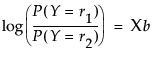where r1 is the first response

or equivalently:

where r1 and r2 are the two responses

For r nominal responses, where

, it fits

sets of linear model parameters of the following form:

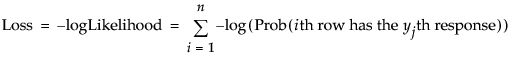
The fitting principal of maximum likelihood means that the βs are chosen to maximize the joint probability attributed by the model to the responses that did occur. This fitting principal is equivalent to minimizing the negative log-likelihood (–LogLikelihood) as attributed by the model:

For example, consider an experiment that was performed on metal ingots prepared with different heating and soaking times. The ingots were then tested for readiness to roll. See Cox (1970). The Ingots.jmp data table in the sample data folder has the experimental results. The categorical variable called ready has values 1 and 0 for readiness and not readiness to roll, respectively.

The Fit Model platform fits the probability of the not readiness (0) response to a logistic cumulative distribution function applied to the linear model with regressors heat and soak:

Probability (not ready to roll) =

The parameters are estimated by minimizing the sum of the negative logs of the probabilities attributed to the observations by the model (maximum likelihood).

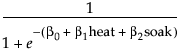
To analyze this model, select Analyze > Fit Model. The ready variable is Y, the response, and heat and soak are the model effects. The count column is the Freq variable. When you click Run, iterative calculations take place. When the fitting process converges, the nominal or ordinal regression report appears. The following sections discuss the report layout and statistical tables, and show examples.