To launch the platform, select Surface Plot from the Graph menu. If there is a data table open, this displays the window in Surface Plot Launch Window. If you do not want to use a data table for drawing surfaces plots, click OK without specifying columns. If there is no data table open, you are presented with the default surface plot shown in Default Surface Plot.
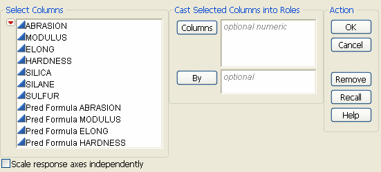
When selected, the Scale response axes independently option gives a separate scale to each response on the plot. When not selected, the axis scale for all responses is the same as the scale for the first item entered in the Columns role.
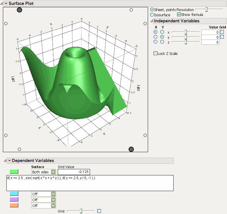
To produce the graph of a mathematical function without any data points, do not fill in any of the roles on the launch window. Simply click OK to get a default plot, as shown in Default Surface Plot.
Select the Show Formula check box to show the formula space.
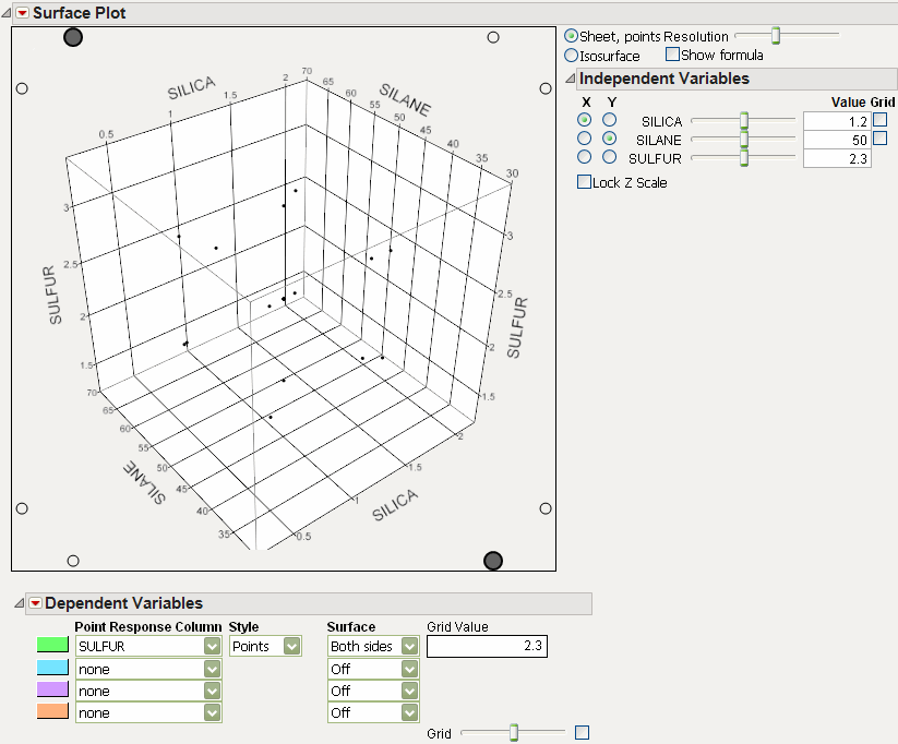
To produce a 3-D scatterplot of points, place the x-, y-, and z-columns in the Columns box. For example, using the Tiretread.jmp data, first select Rows > Clear Row States. Then select Graph > Surface Plot. Assign Silica, Silane, and Sulfur to the Columns role. Click OK.
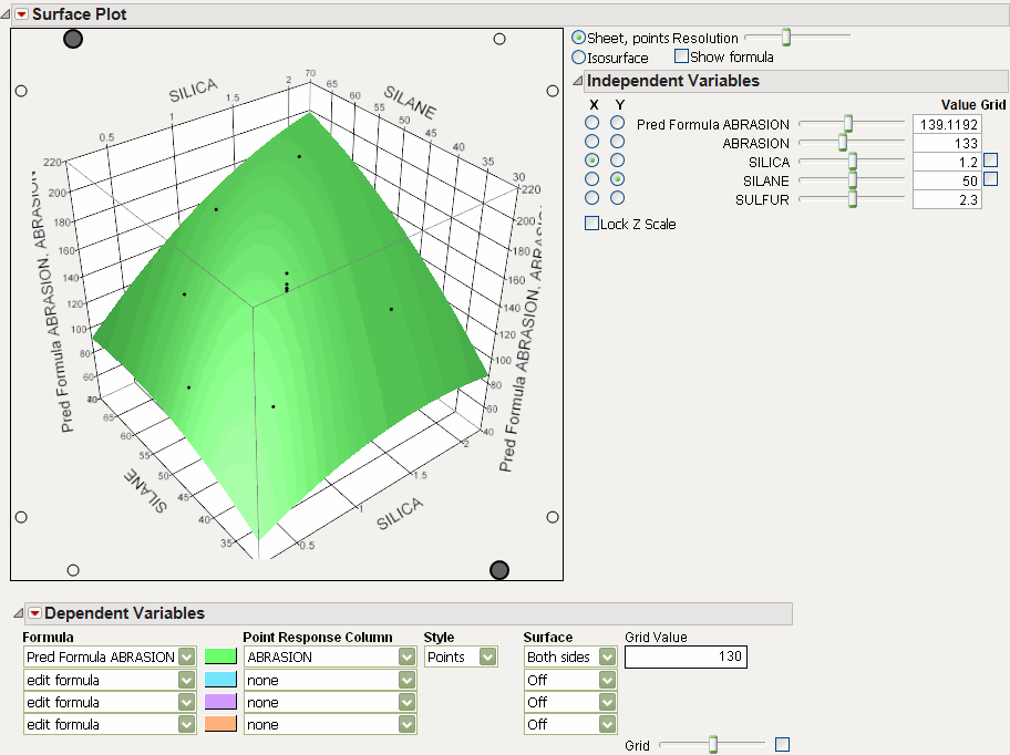
To plot a formula (that is, a formula from a column in the data table), place the column in the Columns box. For example, use the Tiretread.jmp data table and select Graph > Surface Plot. Assign Pred Formula ABRASION to the Columns role. Click OK. You do not have to specify the factors for the plot, because the platform automatically extracts them from the formula.
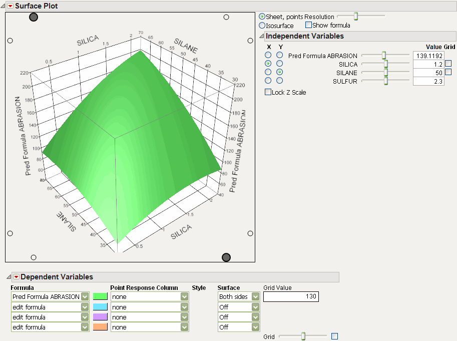
Note that this only plots the prediction surface. To plot the actual values in addition to the formula, assign the ABRASION and Pred Formula ABRASION to the Columns role. Formula and Data Points Launch and Output shows the completed results.
Isosurfaces are the 3-D analogy to a 2-D contour plot. An isosurface requires a formula with three independent variables. The Resolution slider determines the n × n × n cube of points that the formula is evaluated over. The Value slider in the Dependent Variable section selects the isosurface (that is, the contour level) value.
For example, open the Tiretread.jmp data table and run the RSM for 4 Responses script. This produces a response surface model with dependent variables ABRASION, MODULUS, ELONG, and HARDNESS.
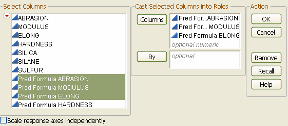
When the report appears, select the Isosurface radio button. Under the Dependent Variables outline node, select Both Sides for all three variables.
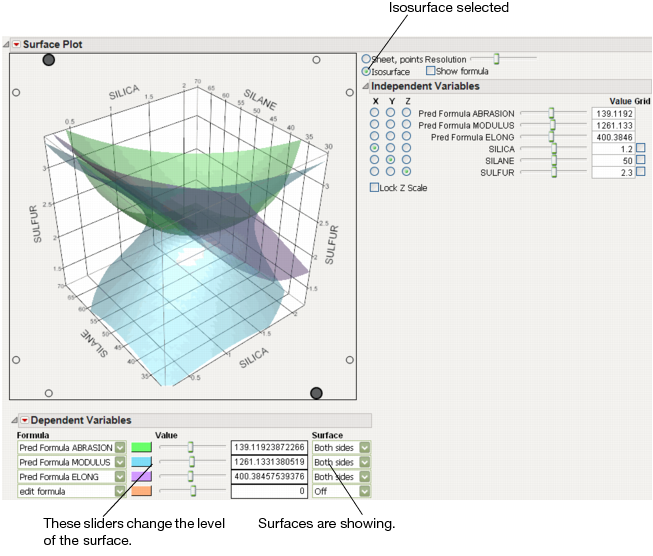
For the tire tread data, one might set the hardness at a fixed minimum setting and the elongation at a fixed maximum setting. Use the MODULUS slider to see which values of MODULUS are inside the limits set by the other two surfaces.