The commands on the Tables menu (and Tabulate on the Analyze menu) summarize and manipulate data tables into the format that you need for graphing and analyzing. This section describes five of these commands:
Create summary tables by using either the Summary or Tabulate commands. The Summary command creates a new data table. As with any data table, you can perform analyses and create graphs from the summary table. The Tabulate command creates a report window with a table of summary data. You can also create a table from the Tabulate report.
|
1.
|
|
2.
|
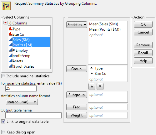
Select Tables > Summary.
|
|
3.
|
|
4.
|
|
5.
|
Click OK.
|
JMP calculates the mean of Sales ($M) and the mean of Profit ($M) for each combination of Type and Size Co.

|
•
|
|
•
|
The N Rows column shows the number of rows from the original table that correspond to each combination of grouping variables. For example, the original data table contains 14 rows corresponding to small computer companies.
|
|
•
|
There is a column for each summary statistic requested. In this example, there is a column for the mean of Sales ($M) and a column for the mean of Profits ($M).
|
|
1.
|
|
2.
|
|
3.
|
|
4.
|
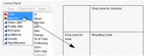
Drag and drop them into the Drop zone for rows.
|
|
5.
|
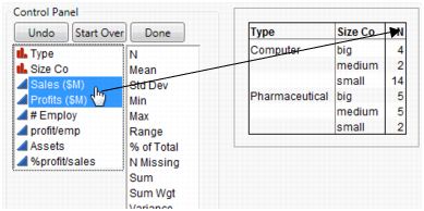
Right-click a heading and select Nest Grouping Columns.
|

|
6.
|
|
7.
|
The final step is to change the sums to means. Right-click Sum (either of them) and select Statistics > Mean.
|
The means are the same as those obtained using the Summary command. Compare Final Tabulation to Summary Table.
|
1.
|
|
2.
|
Select Rows > Row Selection > Select Where.
|
|
3.
|
Select Size Co in the column list box on the left.
|
|
5.
|
Click OK.
|
|
6.
|
|
7.
|
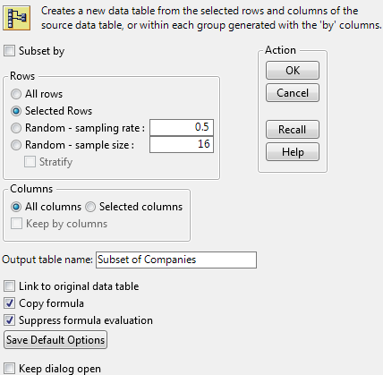
Select Tables > Subset to launch the Subset window.
|
|
8.
|
Select Selected columns to subset only the columns that you selected. You can also customize your subset table further by selecting additional options.
|
|
9.
|
Click OK.
|
|
1.
|
|
2.
|
Select Analyze > Distribution.
|
|
3.
|
|
4.
|
Click OK.
|
Caution: This method creates a linked subset table. This means if you make any changes to the data in the subset table, the corresponding value changes in the source table.
|
1.
|
|
2.
|
Click on Trial1.jmp to make it the active data table.
|
|
3.
|
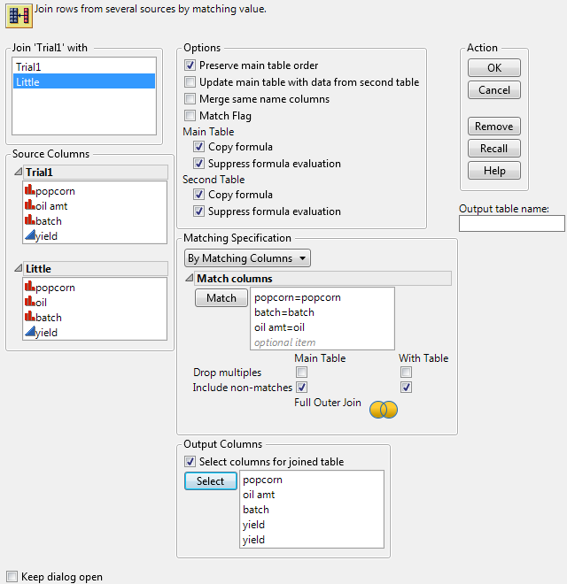
Select Tables > Join.
|
|
4.
|
|
5.
|
|
6.
|
|
7.
|
|
8.
|
Select Include non-matches for both tables.
|
|
9.
|
To avoid duplicate columns, select the Select columns for joined table option.
|
|
10.
|
|
11.
|
|
12.
|
Click OK.
|
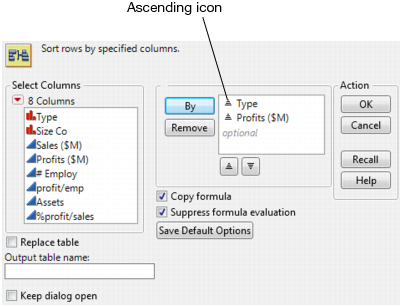
Use the Sort command to sort a data table by one or more columns in the data table. For example, look at financial data for computer and pharmaceutical companies. Suppose that you want to sort the data table by Type, then by Profits ($M). Also, you want Profits ($M) to be in descending order within each Type.
|
1.
|
|
2.
|
|
3.
|
|
4.
|
At this point, both variables are set to be sorted in ascending order. See the ascending icon next to the variables in Sort Ascending Icon.
|
5.
|
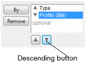
To change Profits ($M) to sort in descending order, select Profits ($M) and click the descending button.
|
|
6.
|
Select the Replace Table check box.
|
When selected, the Replace Table option tells JMP to sort the original data table instead of creating a new table with the sorted values. This option is not available if there are any open report windows created from the original data table. Sorting a data table with open report windows might change how some of the data is displayed in the report window, especially in graphs.
|
7.
|
Click OK.
|