|
2.
|
|
3.
|
Click Run.
|
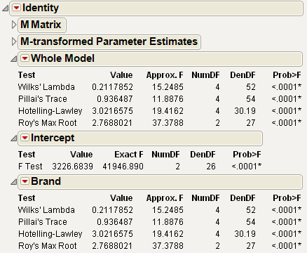
The M Matrix report gives the response design that you specified. The M-transformed Parameter Estimates report gives the original parameter estimates matrix multiplied by the transpose of the M matrix.
Note: Initially in this chapter, the matrix names E and H refer to the error and hypothesis cross products. After specification of a response design, E and H refer to those matrices transformed by the response design, which are actually M´EM and M´HM.
In multivariate fits, the sums of squares due to hypothesis and error are matrices of squares and cross products instead of single numbers. And there are lots of ways to measure how large a value the matrix for the hypothesis sums of squares and cross products (called H or SSCP) is compared to that matrix for the residual (called E). JMP reports the four multivariate tests that are commonly described in the literature. If you are looking for a test at an exact significance level, you may need to go hunting for tables in reference books. Fortunately, all four tests can be transformed into an approximate F test. If the response design yields a single value, or if the hypothesis is a single degree of freedom, the multivariate tests are equivalent and yield the same exact F test. JMP labels the text Exact F; otherwise, JMP labels it Approx. F.
In the golf balls example, there is only one effect so the Whole Model test and the test for Brand are the same, which show the four multivariate tests with approximate F tests. There is only a single intercept with two DF (one for each response), so the F test for it is exact and is labeled Exact F.
The red triangle menus on the Whole Model, Intercept, and Brand reports contain options to generate additional information, which includes eigenvalues, canonical correlations, a list of centroid values, a centroid plot, and a Save command that lets you save canonical variates.
The effect (Brand in this example) popup menu also includes the option to specify contrasts.
The custom test and contrast features are the same as those for regression with a single response. See the Standard Least Squares Report and Options section.
Descriptions of Multivariate Reports describes each Multivariate report (except the Sphericity Test table; see Univariate Tests and the Test for Sphericity).
|
Labels each statistical test in the table. If the number of response function values (columns specified in the M matrix) is 1 or if an effect has only one degree of freedom per response function, the exact F test is presented. Otherwise, the standard four multivariate test statistics are given with approximate F tests: Wilks’ Lambda (Λ), Pillai’s Trace, the Hotelling-Lawley Trace, and Roy’s Maximum Root.
|
|
|
F-values corresponding to the multivariate tests. If the response design yields a single value or if the test is one degree of freedom, this is an exact F test.
|
|
|
•
|
|
•
|
If M yields more than one response the coefficients of each transformation sum to zero.
|
|
•
|
If the sphericity condition is met. The sphericity condition means that the M-transformed responses are uncorrelated and have the same variance. M´ΣM is proportional to an identity matrix, where Σ is the covariance of the Ys.
|
If these conditions hold, the diagonal elements of the E and H test matrices sum to make a univariate sums of squares for the denominator and numerator of an F test. Note that if the above conditions do not hold, then an error message appears. In the case of Golf Balls.jmp, an identity matrix is specified as the M-matrix. Identity matrices cannot be transformed to a full rank matrix after centralization of column vectors and orthonormalization. So the univariate request is ignored.
|
1.
|
|
2.
|
Select Analyze > Fit Model.
|
|
3.
|
|
4.
|
|
5.
|
In the Construct Model Effects panel, select drug. In the Select Columns panel, select dep1. Click Cross.
|
|
6.
|
For Personality, select Manova.
|
|
7.
|
Click Run.
|
|
8.
|
Select the check box next to Univariate Tests Also.
|
|
9.
|
Time should be entered for YName, and Univariate Tests Also should be selected.
|
10.
|
Click OK.
|
The sphericity test checks the appropriateness of an unadjusted univariate F test for the within-subject effects using the Mauchly criterion to test the sphericity assumption (Anderson 1958). The sphericity test and the univariate tests are always done using an orthonormalized M matrix. You interpret the sphericity test as follows:
|
•
|
The univariate F statistic has an approximate F-distribution even without sphericity, but the degrees of freedom for numerator and denominator are reduced by some fraction epsilon (ε). Box (1954), Greenhouse and Geisser (1959), and Huynh-Feldt (1976) offer techniques for estimating the epsilon degrees-of-freedom adjustment. Muller and Barton (1989) recommend the Greenhouse-Geisser version, based on a study of power.
The epsilon adjusted tests in the multivariate report are labeled G-G (Greenhouse-Geisser) or H-F (Huynh-Feldt), with the epsilon adjustment shown in the value column.

