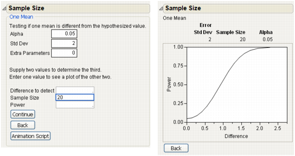
After you click either One Sample Mean, or Two Sample Means in the initial Sample Size selection list (Sample Size and Power Choices), a Sample Size and Power window appears. (See Initial Sample Size and Power Windows for Single Mean (left) and Two Means (right).)
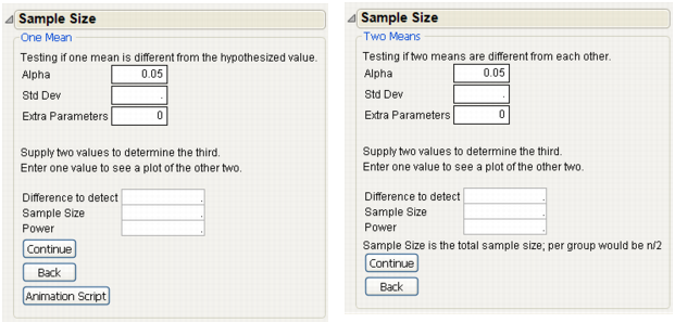
The initial Sample Size and Power window requires values for Alpha, Std Dev (the error standard deviation), and one or two of the other three values: Difference to detect, Sample Size, and Power. The Sample Size and Power platform calculates the missing item. If there are two unspecified fields, a plot is constructed, showing the relationship between these two values:
runs a JSL script that displays an interactive plot showing power or sample size. See the section, Sample Size and Power Animation for One Mean, for an illustration of the animation script.
where μ is the population mean and μ0 is the null mean to test against or is the difference to detect. It is assumed that the population of interest is normally distributed and the true mean is zero. Note that the power for this setting is the same as for the power when the null hypothesis is H0: μ=0 and the true mean is μ0.
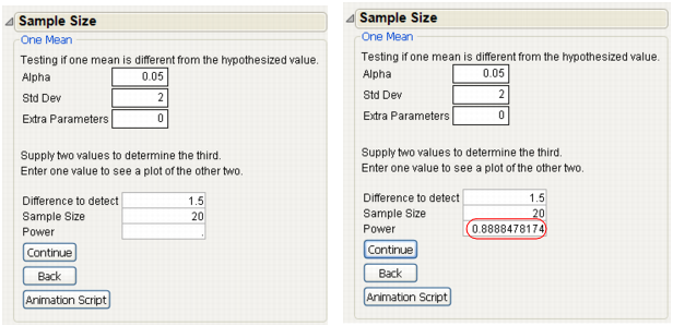
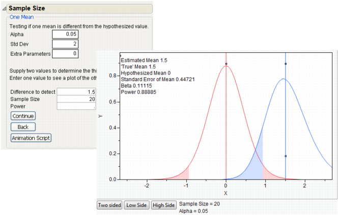
Suppose you are interested in testing the flammability of a new fabric being developed by your company. Previous testing indicates that the standard deviation for burn times of this fabric is 2 seconds. The goal is to detect a difference of 1.5 seconds when alpha is equal to 0.05, the sample size is 20, and the standard deviation is 2 seconds. For this example, μ0 is equal to 1.5. To calculate the power:
|
1.
|
Select DOE > Sample Size and Power.
|
|
2.
|
Click the One Sample Mean button in the Sample Size and Power Window.
|
|
3.
|
Leave Alpha as 0.05.
|
|
4.
|
Leave Extra Parameters as 0.
|
|
5.
|
Enter 2 for Std Dev.
|
|
6.
|
Enter 1.5 as Difference to detect.
|
|
7.
|
Enter 20 for Sample Size.
|
|
8.
|
|
9.
|
Click Continue.
|
The power is calculated as 0.8888478174 and is rounded to 0.89. (See right window in A One-Sample Example.) The conclusion is that your experiment has an 89% chance of detecting a significant difference in the burn time, given that your significance level is 0.05, the difference to detect is 1.5 seconds, and the sample size is 20.
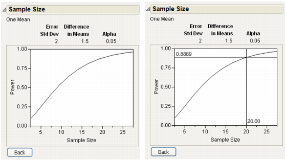
To see a plot of the relationship of Sample Size and Power, leave both Sample Size and Power empty in the window and click Continue.
The plots in A One-Sample Example Plot, show a range of sample sizes for which the power varies from about 0.1 to about 0.95. The plot on the right in A One-Sample Example Plot shows using the crosshair tool to illustrate the example in A One-Sample Example.
When only Sample Size is specified (Plot of Power by Difference to Detect for a Given Sample Size) and Difference to Detect and Power are empty, a plot of Power by Difference appears, after clicking Continue.
Clicking the Animation Script button on the Sample Size and Power window for one mean shows an interactive plot. This plot illustrates the effect that changing the sample size has on power. As an example of using the Animation Script:
|
1.
|
Select DOE > Sample Size and Power.
|
|
2.
|
Click the One Sample Mean button in the Sample Size and Power Window.
|
|
3.
|
Enter 2 for Std Dev.
|
|
4.
|
Enter 1.5 as Difference to detect.
|
|
5.
|
Enter 20 for Sample Size.
|
|
6.
|
Leave Power blank.
|
The Sample Size and Power window appears as shown on the left of Example of Animation Script to Illustrate Power.
|
7.
|
Click Animation Script.
|
Select and drag the square handles to see the changes in statistics based on the positions of the curves. To change the values of Sample Size and Alpha, click on their values beneath the plot.
The Sample Size and Power windows work similarly for one and two sample means; the Difference to Detect is the difference between two means. The comparison is between two random samples instead of one sample and a hypothesized mean.
where μ1 and μ2 are the two population means and D0 is the difference in the two means or the difference to detect. It is assumed that the populations of interest are normally distributed and the true difference is zero. Note that the power for this setting is the same as for the power when the null hypothesis is H0: μ1 − μ2 = 0 and the true difference is D0.
|
1.
|
Select DOE > Sample Size and Power.
|
|
2.
|
Click the Two Sample Means button in the Sample Size and Power Window.
|
|
3.
|
Leave Alpha as 0.05.
|
|
4.
|
Enter 2 for Std Dev.
|
|
5.
|
Leave Extra Parameters as 0.
|
|
6.
|
Enter 1.5 as Difference to detect.
|
|
7.
|
Enter 30 for Sample Size.
|
|
8.
|
Leave Power blank.
|
|
9.
|
Click Continue.
|
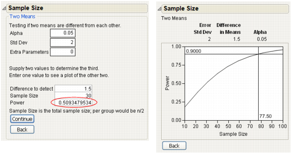
The Power is calculated as 0.51. (See the left window in Plot of Power by Sample Size to Detect for a Given Difference.) This means that you have a 51% chance of detecting a significant difference between the two sample means when your significance level is 0.05, the difference to detect is 1.5, and each sample size is 15.
To have a greater power requires a larger sample. To find out how large, leave both Sample Size and Power blank for this same example and click Continue. Plot of Power by Sample Size to Detect for a Given Difference shows the resulting plot, with the crosshair tool estimating that a sample size of about 78 is needed to obtain a power of 0.9.