To see the options that are available for categorical (nominal and ordinal) variables, see Options for Categorical Variables.
|
The Display Options sub-menu contains the following options:
|
|||
|
|||
|
This option is applicable only if Horizontal Layout is selected.
|
|||
|
The Histogram Options sub-menu contains the following options:
|
|||
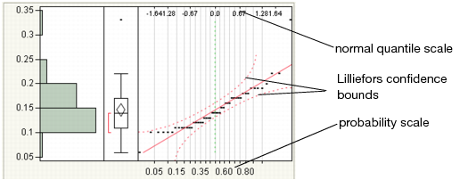
Use the Normal Quantile Plot option to visualize the extent to which the variable is normally distributed. If a variable is normally distributed, the normal quantile plot approximates a diagonal straight line. This type of plot is also called a quantile-quantile plot, or Q-Q plot.
|
•
|
The y-axis shows the column values.
|
|
•
|
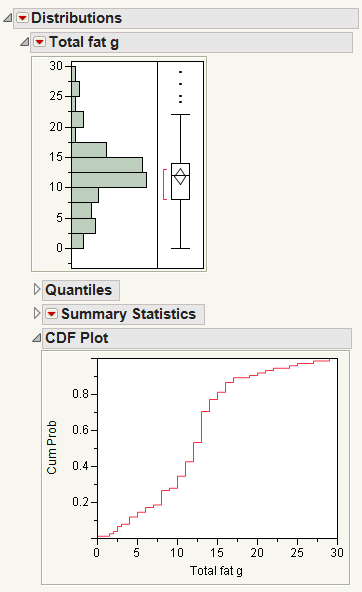
The x-axis shows the empirical cumulative probability for each value.
|
|
•
|
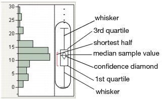
The ends of the box represent the 25th and 75th quantiles, also expressed as the 1st and 3rd quartile, respectively.
|
|
•
|
The difference between the 1st and 3rd quartiles is called the interquartile range.
|
|
•
|
The box has lines that extend from each end, sometimes called whiskers. The whiskers extend from the ends of the box to the outermost data point that falls within the distances computed as follows:
|
|
•
|
The bracket outside of the box identifies the shortest half, which is the most dense 50% of the observations (Rousseuw and Leroy 1987).
|
|
1.
|
|
2.
|
Click Box Plot.
|
|
3.
|
For more details about the Customize Graph window, see the Using JMP book.
The Quantile Box Plot displays specific quantiles from the Quantiles report. If the distribution is symmetric, the quantiles in the box plot are approximately equidistant from each other. At a glance, you can see whether the distribution is symmetric. For example, if the quantile marks are grouped closely at one end, but have greater spacing at the other end, the distribution is skewed toward the end with more spacing. See Quantile Box Plot.
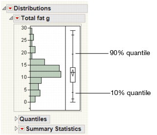
Quantiles are values where the pth quantile is larger than p% of the values. For example, 10% of the data lies below the 10th quantile, and 90% of the data lies below the 90th quantile.
Each line of the plot has a Stem value that is the leading digit of a range of column values. The Leaf values are made from the next-in-line digits of the values. You can see the data point by joining the stem and leaf. In some cases, the numbers on the stem and leaf plot are rounded versions of the actual data in the table. The stem-and-leaf plot actively responds to clicking and the brush tool.
Use the Test Mean window to specify options for and perform a one-sample test for the mean. If you specify a value for the standard deviation, a z-test is performed. Otherwise, the sample standard deviation is used to perform a t-test. You can also request the nonparametric Wilcoxon Signed-Rank test.
Use the Test Mean option repeatedly to test different values. Each time you test the mean, a new Test Mean report appears.
|
Lists the value of the test statistic and the p-values for the two-sided and one-sided alternatives.
|
|
|
(Only appears if the Wilcoxon Signed-Rank test is selected.) Lists the value of the Wilcoxon signed-rank statistic followed by p-values for the two-sided and one-sided alternatives. The test uses the Pratt method to address zero values. This is a nonparametric test whose null hypothesis is that the median equals the postulated value. It assumes that the distribution is symmetric. See Statistical Details for the Wilcoxon Signed Rank Test.
|
|
|
The probability of obtaining an absolute t-value by chance alone that is greater than the observed t-value when the population mean is equal to the hypothesized value. This is the p-value for observed significance of the two-tailed t-test.
|
|
|
The probability of obtaining a t-value greater than the computed sample t ratio by chance alone when the population mean is not different from the hypothesized value. This is the p-value for an upper-tailed test.
|
|
|
The probability of obtaining a t-value less than the computed sample t ratio by chance alone when the population mean is not different from the hypothesized value. This is the p-value for a lower-tailed test.
|
|
Use the Test Std Dev option to perform a one-sample test for the standard deviation (details in Neter, Wasserman, and Kutner 1990). Use the Test Std Dev option repeatedly to test different values. Each time you test the standard deviation, a new Test Standard Deviation report appears.
|
The probability of obtaining a Chi-square value greater than the computed sample Chi-square by chance alone when the population standard deviation is not different from the hypothesized value. This is the p-value for observed significance of a one-tailed t-test.
|
|
|
The probability of obtaining a Chi-square value less than the computed sample Chi-square by chance alone when the population standard deviation is not different from the hypothesized value. This is the p-value for observed significance of a one-tailed t-test.
|
The Confidence Interval options display confidence intervals for the mean and standard deviation. The 0.90, 0.95, and 0.99 options compute two-sided confidence intervals for the mean and standard deviation. Use the Confidence Interval > Other option to select a confidence level, and select one-sided or two-sided confidence intervals. You can also type a known sigma. If you use a known sigma, the confidence interval for the mean is based on z-values rather than t-values.
Use the Save menu commands to save information about continuous variables. Each Save command generates a new column in the current data table. The new column is named by appending the variable name (denoted <colname> in the following definitions) to the Save command name. See Descriptions of Save Commands.
|
Level <colname>
|
||
|
Midpoint <colname>
|
||
|
Ranked <colname>
|
||
|
RankAvgd <colname>
|
If a value is unique, then the averaged rank is the same as the rank. If a value occurs k times, the average rank is computed as the sum of the value’s ranks divided by k.
|
|
|
Prob <colname>
|
For N nonmissing scores, the probability score of a value is computed as the averaged rank of that value divided by N + 1. This column is similar to the empirical cumulative distribution function.
|
|
|
N-Quantile <colname>
|
||
|
Std <colname>
|
||
When you select the Prediction Interval option for a variable, the Prediction Intervals window appears. Use the window to specify the confidence level, the number of future samples, and either a one-sided or two-sided limit.
When you select the Tolerance Interval option for a variable, the Tolerance Intervals window appears. Use the window to specify the confidence level, the proportion to cover, and either a one-sided or two-sided limit. The calculations are based on the assumption that the given sample is selected randomly from a normal distribution.
The Capability Analysis option measures the conformance of a process to given specification limits. When you select the Capability Analysis option for a variable, the Capability Analysis window appears. Use the window to enter specification limits, distribution type, and information about sigma.
Note: To save the specification limits to the data table as a column property, select Save > Spec Limits. When you repeat the capability analysis, the saved specification limits are automatically retrieved.
|
<Distribution type>
|
|
|
Type of process capability indices. See Descriptions of Capability Indices and Computational Formulas.
Note: There is a preference for Capability called Ppk Capability Labeling that labels the long-term capability output with Ppk labels. Open the Preference window (File > Preferences), then select Platforms > Distribution to see this preference.
|
|
|
The PPM value is the Percent column multiplied by 10,000.
|
|
|
Shows the values (represented by Index) of the Benchmark Z statistics. According to the AIAG Statistical Process Control manual, Z represents the number of standard deviation units from the process average to a value of interest such as an engineering specification. When used in capability assessment, Z USL is the distance to the upper specification limit and Z LSL is the distance to the lower specification limit. See Statistical Details for Capability Analysis.
|
|