Neural Network Diagram shows a two-layer neural network with three X variables and one Y variable. In this example, the first layer has two nodes, and each node is a function of all three nodes in the second layer. The second layer has three nodes, and all nodes are a function of the three X variables. The predicted Y variable is a function of both nodes in the first layer.
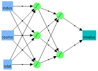
The functions applied at the nodes of the hidden layers are called activation functions. The activation function is a transformation of a linear combination of the X variables. For more details about the activation functions, see Hidden Layer Structure.
|
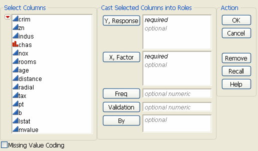
Choose a validation column. For more information, see Validation Method. If you click the Validation button with no columns selected in the Select Columns list, you can add a validation column to your data table. For more information about the Make Validation Column utility, see Basic Analysis.
|
|
|
For a continuous variable, missing values are replaced by the mean of the variable. Also, a missing value indicator, named <colname> Is Missing, is created and included in the model. If a variable is transformed using the Transform Covariates fitting option on the Model Launch window, missing values are replaced by the mean of the transformed variable.
|
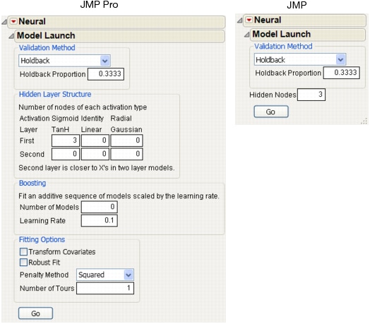
After you click Go to fit a model, you can reopen the Model Launch Dialog and change the settings to fit another model.
|
•
|
The training set is the part that estimates model parameters.
|
|
•
|
The validation set is the part that estimates the optimal value of the penalty, and assesses or validates the predictive ability of the model.
|
|
•
|
The test set is a final, independent assessment of the model’s predictive ability. The test set is available only when using a validation column. See Validation Methods.
|
The training, validation, and test sets are created by subsetting the original data into parts. Validation Methods describes several methods for subsetting a data set.
The functions applied at the nodes of the hidden layers are called activation functions. An activation function is a transformation of a linear combination of the X variables. Activation Functions describes the three types of activation functions.
 where x is a linear combination of the X variables.
|
|
|
where x is a linear combination of the X variables.
|
The learning rate must be 0 < r ≤ 1. Learning rates close to 1 result in faster convergence on a final model, but also have a higher tendency to overfit data. Use learning rates close to 1 when a small Number of Models is specified.
Fitting Options describes the model fitting options that you can specify.
The penalty is  , where λ is the penalty parameter, and p( ) is a function of the parameter estimates, called the penalty function. Validation is used to find the optimal value of the penalty parameter.
|
|
||
|
|
||
 |
||