A leverage plot for an effect shows the impact of adding this effect to the model, given the other effects already in the model. For illustration, consider the construction of an effect leverage plot for a single continuous effect X. See X Axis Scaling for information about the scaling of the x-axis in more general situations.
The effect leverage plot for X is essentially a scatterplot of the X-residuals against the Y-residuals (Whole Model and Effect Leverage Plots). To help interpretation and comparison with other plots that you might construct, JMP adds the mean of Y to the Y-residuals and the mean of X to the X-residuals. The translated Y-residuals are called the Y Leverage Residuals and the translated X-residuals are called X Leverage values. The points on the Effect Leverage plots are these X Leverage and Y Leverage Residual pairs.
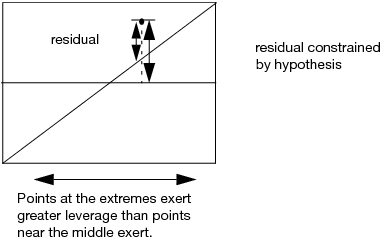
Illustration of a Generic Leverage Plot shows how residuals are depicted in the leverage plot. The distance from a point to the line of fit is the residual for a model that includes the effect. The distance from the point to the horizontal line is what the residual error would be without the effect in the model. In other words, the mean line in the leverage plot represents the model where the hypothesized value of the parameter (effect) is constrained to zero.
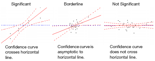
Confidence curves for the line of fit are shown on leverage plots. These curves provide a visual indication of whether the test of interest is significant at the 5% level (or at the Set Alpha Level that you specified in the Fit Model launch window). If the confidence region between the curves contains the horizontal line representing the hypothesis, then the effect is not significant. If the curves cross the line, the effect is significant. See the examples in Comparison of Significance Shown in Leverage Plots.
If the modeling type of a predictor X is continuous, then the x-axis is scaled in terms of the units of the X. The x-axis range mirrors the range of X values. The slope of the line of fit in the leverage plot is the parameter estimate for X. See the left illustration in Whole Model and Effect Leverage Plots.
If the effect is nominal or ordinal, or if the effect is a complex effect such as an interaction, then the x-axis cannot represent the values of the effect directly. In this case the x-axis is scaled in units of the response, and the line of fit is a diagonal with a slope of 1. The Whole Model leverage plot, where the hypothesis of interest is that all parameter values are zero, uses this scaling. (See Leverage Plot Details.) For this plot, the x-axis is scaled in terms of predicted response values for the whole model, as illustrated by the right-hand plot in Whole Model and Effect Leverage Plots.
The term leverage is used because these plots help you visualize the influence of points on the test for including the effect in the model. A point that is horizontally distant from the center of the plot exerts more influence on the effect test than does a point that is close to the center. Recall that the test for an effect involves comparing the sum of squared residuals to the sum of squared residuals of the model with that effect removed. At the extremes, the differences of the residuals before and after being constrained by the hypothesis tend to be comparatively larger. Therefore, these residuals tend to have larger contributions to the sums of squares for that effect’s hypothesis test.
Multicollinearity is a condition where two or more predictors are highly related, or more technically, involved in a nearly linear dependent relationship. When multicollinearity is present, standard errors can be inflated and parameters estimates can be unstable. If an effect is collinear with other predictors, the y-axis values are very close to the horizontal line at the mean, because the effect brings no new information. Because of the dependency, the x-axis values also tend to cluster toward the middle of the plot. This situation indicates that the slope of the line of fit is unstable.
The Plot Effect Leverage option produces a leverage plot for each effect in the model. In addition, the Actual by Predicted plot can be considered to be a leverage plot. This plot lets you visualize the test that all the parameters in the model (except the intercept) are zero. The same test is conducted analytically in the Analysis of Variance report. (See Leverage Plot Details for details about this plot.)
|
1.
|
|
2.
|
Select Analyze > Fit Model.
|
|
3.
|
|
4.
|
|
5.
|
Click Run.
|
The Whole Model Actual by Predicted Plot and the effect Leverage Plot for height are shown in Whole Model and Effect Leverage Plots. The Whole Model plot, on the left, tests for all effects. You can infer that the model is significant because the confidence curves cross the horizontal line at the mean of the response, weight. The Leverage Plot for height, on the right, also shows that height is significant, even with age and sex in the model. Neither plot suggests concerns relative to influential points or multicollinearity.
The Press, or prediction error sum of squares, statistic is an estimate of prediction error computed using leave-one-out cross validation. In leave-one-out cross validation, each observation, in turn, is removed. Consider a specific observation. The model is fit with that observation withheld and then a predicted value is obtained for that observation. The residual for that observation is computed. This procedure is applied to all observations and the residuals are squared and summed to give the Press value.
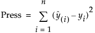
where n is the number of observations, yi is the observed response value for the ith observation, and  is the predicted response value for the ith observation. These values are based on a model fit without including that observation.