In JMP’s implementation, the Profiler first looks at the factor and response variables to see whether there is a Sigma column property (a specification for the standard deviation of the column, accessed through the Cols > Column Info dialog box). If the property exists, then the Prop of Error Bars command becomes accessible in the Prediction Profiler drop-down menu. This displays the 3σ interval that is implied on the response due to the variation in the factor.
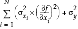
where σy is the user-specified sigma for the response column, and σx is the user-specified sigma for the factor column.
centered, with δ=xrange/10000
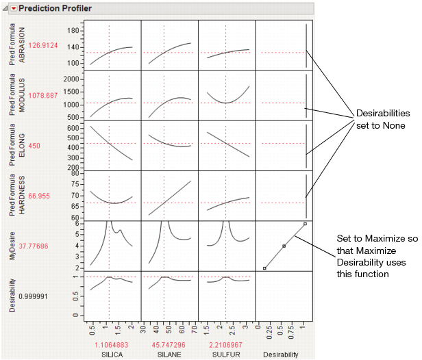
First, create a column called MyDesire that contains the above formula. Then, select Graph > Profiler to launch the platform. Select all the Pred Formula columns and the MyDesire column and select Y, Prediction Formula. Turn on the desirability functions by selecting Desirability Functions from the red triangle menu. All the desirability functions for the individual effects must be turned off. To do this, first double-click in a desirability plot window, then select None in the window that appears (Selecting No Desirability Goal). Set the desirability for MyDesire to be maximized.
For example, when Fit Model fits a logistic regression for two levels (say A and B), the end formulas (Prob[A] and Prob[B]) are functions of the Lin[x] column, which itself is a function of another column x. If Expand Intermediate Formulas is selected, then when Prob[A] is profiled, it is with reference to x, not Lin[x].
To enter linear constraints via the red triangle menu, select Alter Linear Constraints from either the Prediction Profiler or Custom Profiler red triangle menu.
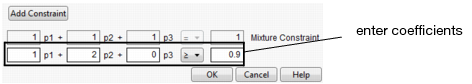
Choose Add Constraint from the resulting window, and enter the coefficients into the appropriate boxes. For example, to enter the constraint p1 + 2*p2 ≥ 0.9, enter the coefficients as shown in Enter Coefficients. As shown, if you are profiling factors from a mixture design, the mixture constraint is present by default and cannot be modified.
After you click OK, the Profiler updates the profile traces, and the constraint is incorporated into subsequent analyses and optimizations.
Constraints added in one profiler are not accessible by other profilers until saved. For example, if constraints are added under the Prediction Profiler, they are not accessible to the Custom Profiler. To use the constraint, you can either add it under the Custom Profiler red triangle menu, or use the Save Linear Constraints command described in the next section.
If you add constraints in one profiler and want to make them accessible by other profilers, use the Save Linear Constraints command, accessible through the platform red triangle menu. For example, if you created constraints in the Prediction Profiler, choose Save Linear Constraints under the Prediction Profiler red triangle menu. The Save Linear Constraints command creates or alters a Table Script called Constraint. An example of the Table Property is shown in Constraint Table Script.
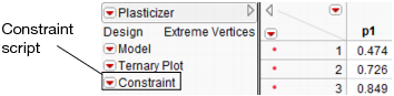
The Constraint Table Property is a list of the constraints, and is editable. It is accessible to other profilers, and negates the need to enter the constraints in other profilers. To view or edit Constraint, right-click the red triangle menu and select Edit. The content of the constraint from Enter Coefficients is shown below in Example Constraint.
The Constraint Table Script can be created manually by choosing New Script from the red triangle menu beside a table name.
Note: When creating the Constraint Table Script manually, the spelling must be exactly “Constraint”. Also, the constraint variables are case sensitive and must match the column name. For example, in Example Constraint, the constraint variables are p1 and p2, not P1 and P2.