The response can be either continuous, or categorical (nominal or ordinal). If Y is categorical, then it is fitting the probabilities estimated for the response levels, minimizing the residual log-likelihood chi-square [2*entropy]. If the response is continuous, then the platform fits means, minimizing the sum of squared errors.
The factors can be either continuous, or categorical (nominal or ordinal). If an X is continuous, then the partition is done according to a splitting “cut” value for X. If X is categorical, then it divides the X categories into two groups of levels and considers all possible groupings into two levels.
where the adjusted p-value is calculated in a complex manner that takes into account the number of different ways splits can occur. This calculation is very fair compared to the unadjusted p-value, which favors Xs with many levels, and the Bonferroni p-value, which favors Xs with small numbers of levels. Details on the method are discussed in a white paper “Monte Carlo Calibration of Distributions of Partition Statistics” found on the JMP website www.jmp.com.
For categorical responses, the G2 (likelihood-ratio chi-square) is shown in the report. This is actually twice the [natural log] entropy or twice the change in the entropy. Entropy is Σ -log(p) for each observation, where p is the probability attributed to the response that occurred.
is the predicted probability for that node of the tree. The method for calculating Prob for the ith response level at a given node is as follows:
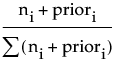
where the summation is across all response levels; ni is the number of observations at the node for the ith response level; and priori is the prior probability for the ith response level, calculated as
where pi is the priori from the parent node, Pi is the Probi from the parent node, and λ is a weighting factor currently set at 0.9.