Statistical Details for Multivariate Control Charts

This section contains statistical details for individual data, sub-grouped data, additivity, and change point detection.

Statistical Details for Individual Data

Consider measurements that are not sub-grouped, that is, where the natural subgroup size is one. Denote the number of samples by n and the number of characteristics measured by p. Then the T2 statistic is defined as follows:

where:

Xi is the column vector of p measurements for the ith sample

X is the sample mean of the Xi

S is the sample covariance matrix for the Xi

These are the points plotted on the multivariate control chart.

When computing control limits based on historical data (Step 1), the UCL is based on the beta distribution. Specifically, the UCL is defined as follows:

where:

p is number of variables

n is the sample size

Once you have specified targets (Step 2), new observations are independent of the historical statistics. In this case, the UCL is a function of the F-distribution and partially depends on the number of observations in the data from which the targets are calculated.

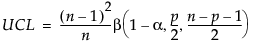
If n is less than or equal to 100, the UCL is defined as:

If n is greater than 100, the UCL is defined as:

In both equations,

p is number of variables

n is the sample size for the data from which the targets were calculated

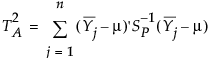
Statistical Details for Sub-Grouped Data

Consider the case where p characteristics are monitored and where m subgroups of size n are obtained. A value of the T2 statistic is plotted for each subgroup. The T2 statistic for the ith subgroup is defined as follows:

where:

Xi is the mean of the n column vectors of p measurements for the ith sample

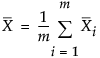is the overall mean of the observations

Si is the sample covariance matrix for the n observations in the ith subgroup

is the mean of the within-subgroup covariance matrices

Using historical data (Step 1), before specifying targets, the UCL is defined as follows:

where:

p is number of characteristics

n is the sample size for each subgroup

m is the number of subgroups

When you compare current data to historical targets, the UCL is defined as follows:

where:

p is number of variables

n is the sample size for each subgroup

m is the number of subgroups

Statistical Details for Additivity

When a sample of mn independent normal observations is grouped into m rational subgroups of size n, the distance between the mean Yj of the jth subgroup and the expected value μ is T2M. Note that the components of the T2 statistic are additive, much like sums of squares. In other words, the following computation is true:

Let T2M represent the distance from a target value:

The internal variability is defined as follows:

The overall variability is defined as follows:

Statistical Details for Change Point Detection

Suppose that there are m independent observations from a multivariate normal distribution of dimensionality p, such that the following equation is true:

where xi is an individual observation, and Np(μi,Σi) represents a multivariate normally distributed mean vector and covariance matrix, respectively.

If a distinct change occurs in the mean vector, the covariance matrix, or both, after m1 observations, all observations through m1 have the same mean vector and the same covariance matrix (μa,Σa). Similarly, all ensuing observations, beginning with m1 + 1, have the same mean vector and covariance matrix (μb,Σb). If the data are from an in-control process, then μa = μb and Σa = Σb for all values of m, and the parameters of the in-control process can be estimated directly from the data.

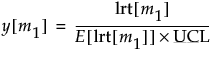
A likelihood ratio test approach is used to determine changes or a combination of changes in the mean vector and covariance matrix. The likelihood ratio statistic is plotted for all possible m1 values, and an appropriate Upper Control Limit (UCL) is chosen. The location (observation or row number) of the maximum test statistic value corresponds to the maximum likelihood location of only one shift, assuming that exactly one change (or shift) occurred.

The log of the likelihood function is maximized for the first m1 observations, as follows:

where |S1| is the maximum likelihood estimate of the covariance matrix for the first m1 observations, and the rank of S1 is defined as k1 = Min[p,m1-1], where p is the dimensionality of the matrix.

The log-likelihood function for the subsequent m2 = m - m1 observations is l2, and is calculated similarly to l0, which is the log-likelihood function for all m observations.

The sum l1 + l2 is the likelihood that assumes a possible shift at m1, and is compared with the likelihood l0, which assumes no shift. If l0 is substantially smaller than l1 + l2, the process is assumed to be out of control.

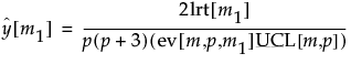
The log-likelihood ratio, multiplied by two, is defined as follows:

The log-likelihood ratio has a chi-squared distribution, asymptotically, with the degrees of freedom equal to p(p + 3)/2. Large log-likelihood ratio values indicate that the process is out-of-control.

Divide the above equation (the log-likelihood ratio, multiplied by two) by its expected value. That value is determined from simulation and by the UCL, yields an upper control limit of one on the control chart. Therefore, the control chart statistic becomes the following:

and, after dividing by p(p+3)/2, this equation yields the expected value:

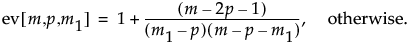
The intercept in the above equation is as follows:

and the slope is as follows:

When p = 2, the value of ev[m,p,m1] when m1 or m2 = 2 is 1.3505. Note that the above formulas are not accurate for p > 12 or m < (2p + 4). In such cases, simulation should be used.

With step 1 control charts, it is useful to specify the upper control limit (UCL) as the probability of a false out-of-control signal. An approximate UCL where the false out-of-control signal is approximately 0.05 and is dependent upon m and p, is given as follows:

The approximate control chart statistic is then given as follows: