Note: Many distributions in the Life Distribution platform are parameterized by location and scale. For lognormal fits, the median is also provided. A threshold parameter is also included in threshold distributions. Location corresponds to μ, scale corresponds to σ, and threshold corresponds to γ.
 ,
,
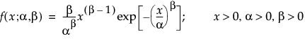
The Weibull distribution can be used to model failure time data with either an increasing or a decreasing hazard rate. It is used frequently in reliability analysis because of its tremendous flexibility in modeling many different types of data, based on the values of the shape parameter, β. This distribution has been successfully used for describing the failure of electronic components, roller bearings, capacitors, and ceramics. Various shapes of the Weibull distribution can be revealed by changing the scale parameter, α, and the shape parameter, β. The Weibull pdf and cdf are commonly represented as follows:
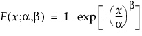 ,
,where α is a scale parameter, and β is a shape parameter. The Weibull distribution is particularly versatile because it reduces to an exponential distribution when β = 1. An alternative parameterization commonly used in the literature and in JMP is to use σ as the scale parameter and μ as the location parameter. These are easily converted to an α and β parameterization by
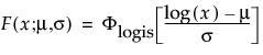
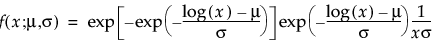
The pdf and the cdf of the Weibull distribution are also expressed as a log-transformed smallest extreme value distribution (SEV). This uses a location scale parameterization, with μ = log(α) and σ = 1/β,
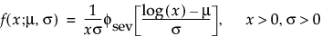
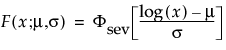
are the pdf and cdf, respectively, for the standardized smallest extreme value (μ = 0, σ = 1) distribution.
 ,
,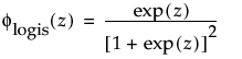
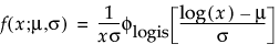
are the pdf and cdf, respectively, for the standardized logistic or logis distribution(μ = 0, σ = 1).

are the pdf and cdf, respectively, for the standardized largest extreme value LEV(μ = 0, σ = 1) distribution.
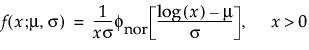
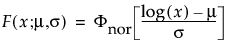
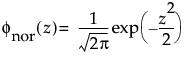
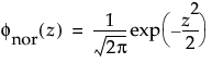
The normal distribution is the most widely used distribution in most areas of statistics because of its relative simplicity and the ease of applying the central limit theorem. However, it is rarely used in reliability. It is most useful for data where μ > 0 and the coefficient of variation (σ/μ) is small. Because the hazard function increases with no upper bound, it is particularly useful for data exhibiting wear-out failure. Examples include incandescent light bulbs, toaster heating elements, and mechanical strength of wires. The pdf and cdf are:


This non-symmetric (left-skewed) distribution is useful in two cases. The first case is when the data indicate a small number of weak units in the lower tail of the distribution (the data indicate the smallest number of many observations). The second case is when σ is small relative to μ, because probabilities of being less than zero, when using the SEV distribution, are small. The smallest extreme value distribution is useful to describe data whose hazard rate becomes larger as the unit becomes older. Examples include human mortality of the aged and rainfall amounts during a drought. This distribution is sometimes referred to as a Gumbel distribution. The pdf and cdf are:
are the pdf and cdf, respectively, for the standardized smallest extreme value, SEV(μ = 0, σ = 1) distribution.
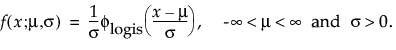
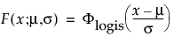
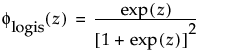
are the pdf and cdf, respectively, for the standardized logistic or logis distribution (μ = 0, σ = 1).
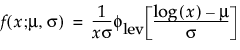
This right-skewed distribution can be used to model failure times if σ is small relative to μ > 0. This distribution is not commonly used in reliability but is useful for estimating natural extreme phenomena, such as a catastrophic flood heights or extreme wind velocities. The pdf and cdf are:
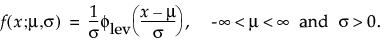
are the pdf and cdf, respectively, for the standardized largest extreme value LEV(μ = 0, σ = 1) distribution.
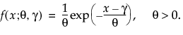
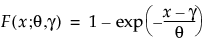
where θ is a scale parameter and γ is both the threshold and the location parameter. Reliability analysis frequently uses the one-parameter exponential distribution, with γ = 0. The exponential distribution is useful for describing failure times of components exhibiting wear-out far beyond their expected lifetimes. This distribution has a constant failure rate, which means that for small time increments, failure of a unit is independent of the unit’s age. The exponential distribution should not be used for describing the life of mechanical components that can be exposed to fatigue, corrosion, or short-term wear. This distribution is, however, appropriate for modeling certain types of robust electronic components. It has been used successfully to describe the life of insulating oils and dielectric fluids (Nelson, 1990, p. 53).
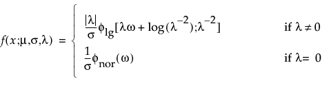
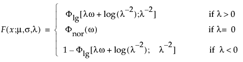
are the pdf and cdf, respectively, for the log-gamma variable and κ > 0 is a shape parameter. The standardized distributions above are dependent upon the shape parameter κ.
Note: In JMP, the shape parameter, λ, for the generalized gamma distribution is bounded between [-12,12] to provide numerical stability.
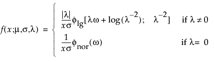
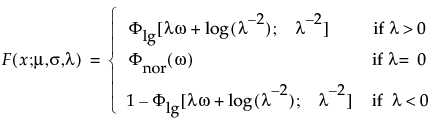
are the pdf and cdf, respectively, for the standardized log-gamma variable and κ > 0 is a shape parameter.
The standardized distributions above are dependent upon the shape parameter κ. Meeker and Escobar (chap. 5) give a detailed explanation of the extended generalized gamma distribution.
Note: In JMP, the shape parameter, λ, for the generalized gamma distribution is bounded between [-12,12] to provide numerical stability.
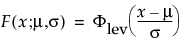
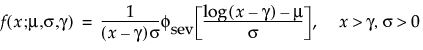
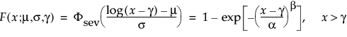
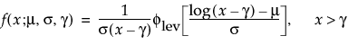
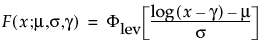
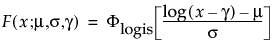
Threshold Distributions are log-location-scale distributions with threshold parameters. Some of the distributions above are generalized by adding a threshold parameter, denoted by γ. The addition of this threshold parameter shifts the beginning of the distribution away from 0. Threshold parameters are sometimes called shift, minimum, or guarantee parameters because all units survive the threshold. Note that while adding a threshold parameter shifts the distribution on the time axis, the shape, and spread of the distribution are not affected. Threshold distributions are useful for fitting moderate to heavily shifted distributions. The general forms for the pdf and cdf of a log-location-scale threshold distribution are:
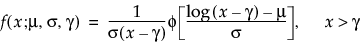

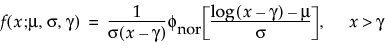
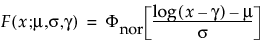
where φ and Φ are the pdf and cdf, respectively, for the specific distribution. Examples of specific threshold distributions are shown below for the Weibull, lognormal, Fréchet, and loglogistic distributions, where, respectively, the SEV, Normal, LEV, and logis pdfs and cdfs are appropriately substituted.
are the pdf and cdf, respectively, for the standardized smallest extreme value, SEV(μ = 0, σ = 1) distribution.
are the pdf and cdf, respectively, for the standardized largest extreme value LEV(μ = 0, σ = 1) distribution.
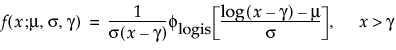

are the pdf and cdf, respectively, for the standardized logistic or logis distribution (μ = 0, σ = 1).
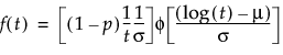
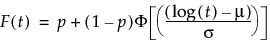
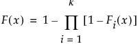
Zero-inflated distributions are used when some proportion (p) of the data fail at t = 0. When the data contain more zeros than expected by a standard model, the number of zeros is inflated. When the time-to-event data contain zero as the minimum value in the Life Distribution platform, four zero-inflated distributions are available. These distributions include:
p is the proportion of zero data values,
t is the time of measurement for the lifetime event,
μ and σ are estimated by calculating the usual maximum likelihood estimations after removing zero values from the original data,
φ(z) and Φ(z) are the density and cumulative distribution function, respectively, for a standard distribution. For example, for a Weibull distribution,
See Lawless (2003, p 34) for a more detailed explanation of using zero-inflated distributions. Substitute p = 1 - p and S1(t) = 1 - Φ(t) to obtain the form shown above.
See Tobias and Trindade (1995, p 232) for additional information about reliability distributions. This reference gives the general form for mixture distributions. Using the parameterization in Tobias and Trindade, the form above can be found by substituting α = p, Fd(t) = 1, and FN(t) = Φ(t).
|
•
|
|
1.
|
|
2.
|
|
3.
|
|
4.
|
|
5.
|
Select Likelihood as the Confidence Interval Method.
|
|
6.
|
Select Allow failure mode to use fixed parameter models.
|
|
7.
|
Click OK.
|
|
9.
|
Select Fix Parameter from the red triangle next to Parametric Estimate - Weibull.
|
|
10.
|
Select Weibull beta and type 2.
|
|
11.
|
Click Update.
|
|
13.
|
Deselect Omit for Cause 1.
|
|
14.
|
For the distribution for Cause 1, select Fixed Parameter Weibull.
|
|
15.
|
Click Update Model.
|
The steps for specifying a Bayesian model for a cause are similar to those described in Specify a Fixed Parameter Model as a Distribution for a Cause. Define the model in the desired Bayesian Estimation report found in the corresponding Parametric Estimate outline under Statistics in the Life Distribution report for the individual cause. See Bayesian Estimation - <Distribution Name>.
To incorporate a Bayesian model into the aggregated model, non-Bayesian distributions for other causes must be amenable to a simulation-based framework. For example, suppose that a model has two failure causes. One is modeled using a Weibull distribution and the other using a Bayesian approach for estimating the parameters of a second Weibull. The parameters for the first Weibull distribution, denoted by the vector θ1, are estimated using maximum likelihood. The parameters for the second Weibull, θ2, are estimated using the Bayesian approach.
|
•
|
The steps for specifying a Weibayes model for a cause are similar to those described in Specify a Fixed Parameter Model as a Distribution for a Cause. Select the Fix Parameter option in the Parametric Estimate - Weibull outline under Statistics in the Life Distribution report for the cause. In the Fix Parameter report, check the Weibayes option. The Weibayes model is treated as a Bayesian model and a bootstrap sample is drawn from the posterior distribution of the parameter alpha. See Liu and Wang (2013).
To obtain an estimate of the mean remaining life at time t, m samples are drawn from the aggregated distribution conditioned on survival to time t. Their average is computed.
To compute the confidence interval, n samples of parameter estimates are drawn from either the asymptotic distributions of the MLEs, or the posterior distributions derived using Bayesian inference. For each sample of parameter values, an aggregated distribution is formed, from which m samples are drawn to compute a mean remaining life. The samples of n mean remaining life values are used to construct the confidence interval.
|
‒
|
If the observation y is not censored, the saved value is given by
|
