Examine the Response Surface Report
1. Click the Response Y red triangle and select Estimates > Show Prediction Expression.
Figure 4.13 Prediction Expression
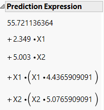
Tip: The Prediction Expression is the prediction formula. You can also obtain this formula by selecting Save Columns > Prediction Formula.
In the following steps, you can refer to the prediction expression to see the model coefficients.
2. Open the Response Surface report and then the Canonical Curvature report.
Figure 4.14 Response Surface Report
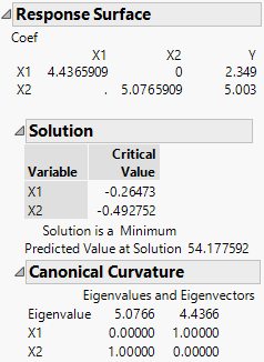
The first table gives the second-order model coefficients in matrix form. The coefficient of X1*X1 is 4.4365909, the coefficient of X2*X2 is 5.0765909, and the coefficient of X1*X2 is 0. The coefficients of the linear effects, 2.349 for X1 and 5.003 for X2, are given in the column labeled Y.
The Solution report shows the critical values. These are the values where a maximum, a minimum, or a saddle point occur. In this example, the Solution report indicates that the response surface achieves a minimum of 54.18 at the critical value, where X1 = -0.265 and X2 = -0.493.
The Canonical Curvature report shows the eigenstructure of the matrix of second-order parameter estimates. The eigenstructure is useful for identifying the shape and orientation of the curvature. See Canonical Curvature Report in the Standard Least Squares Report and Options section.
In this example, both eigenvalues are positive, which indicates that the surface achieves a minimum. The direction of greatest curvature corresponds to the largest eigenvalue (5.0766). That direction is defined by the corresponding eigenvector components. For the first direction, X2, with an eigenvector value of 1.00, determines the direction. The second direction is determined by X1, also with an eigenvector value of 1.00.