Example of Gaussian Process
This example uses data from a space filling design in two variables with a deterministic equation for Y (the response). You can use the Gaussian Process platform to find the explanatory power of X1 and X2 on Y. You can view the equation for Y in the column formula.
1. Select Help > Sample Data Library and open 2D Gaussian Process Example.jmp.
2. Select Analyze > Specialized Modeling > Gaussian Process.
3. Select X1 and X2 and click X.
4. Select Y and click Y
5. Select Correlation Type > Cubic.
6.  Deselect Fast GASP.
7. Click OK.
Figure 16.2 Gaussian Process Report
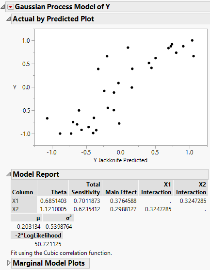
Note: The estimated parameters can be different due to different starting points in the minimization routine, the choice of correlation type, and the inclusion of a nugget parameter.
Now, visualize the fitted surface compared to the original surface.
8. Click the red triangle next to Gaussian Process Model of Y and select Save Prediction Formula.
9. Select Graph > Surface Plot.
10. Select X1 through Y Prediction Formula and click Columns.
11. Click OK.
12. In the Surface column, select Both sides for the Y Prediction Formula.
Figure 16.3 3D Surface Plot of the Actual and Predicted Ys
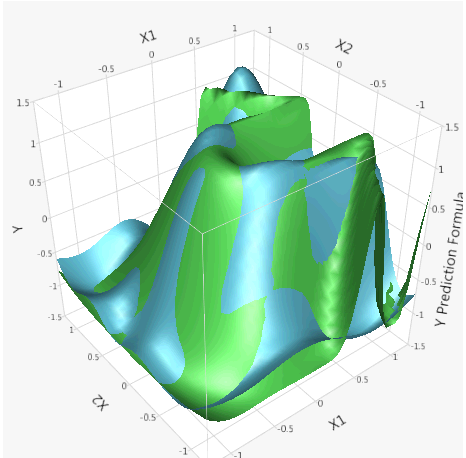
The two surfaces are similar. The impact of X1 and X2 on the response Y can be visualized. You can rotate the plot to view it from different angles. Marginal plots are another tool to use to understand the impact of the factors on the response.