Additional Example of Measurement Systems Analysis
In this example, three operators have measured a single characteristic twice on each of six wafers. Perform a detailed analysis to find out how well the measurement system is performing.
Perform the Initial Analysis
1. Select Help > Sample Data Library and open Variability Data/Wafer.jmp.
2. Select Analyze > Quality and Process > Measurement Systems Analysis.
3. Assign Y to the Y, Response role.
4. Assign Wafer to the Part, Sample ID role.
5. Assign Operator to the X, Grouping role.
Notice that the MSA Method is set to EMP, the Chart Dispersion Type is set to Range, and the Model Type is set to Crossed.
6. Click OK.
Figure 4.8 Average and Range Charts
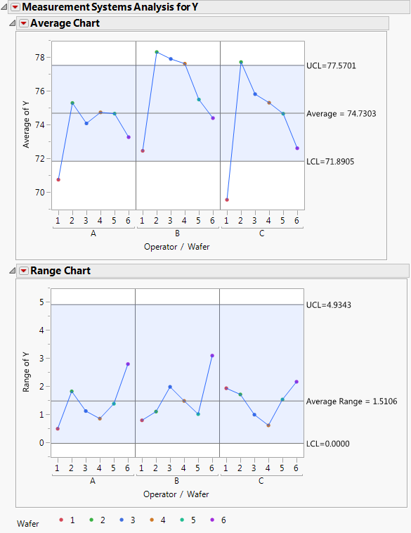
The Average Chart shows that some of the average part measurements fall beyond the control limits. This is desirable, indicating measurable part-to-part variation.
The Range Chart shows no points that fall beyond the control limits. This is desirable, indicating that the operator measurements are consistent within part.
Examine Interactions
Take a closer look for interactions between operators and parts. Click the red triangle next to Measurement Systems Analysis for Y and select Parallelism Plots.
Figure 4.9 Parallelism Plot
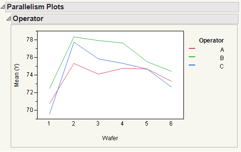
Looking at the parallelism plot by operator, you can see that the lines are relatively parallel and that there is only some minor crossing.
Examine Operator Consistency
Take a closer look at the variance between operators. Click the red triangle next to Measurement Systems Analysis for Y and select Test-Retest Error Comparison.
Figure 4.10 Test-Retest Error Comparison
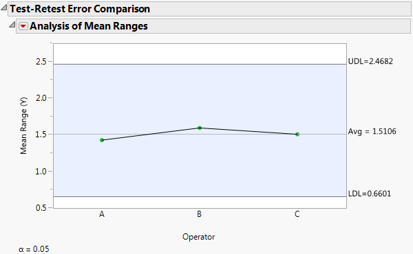
Looking at the Test-Retest Error Comparison, you can see that none of the operators have a test-retest error that is significantly different from the overall test-retest error. The operators appear to be measuring consistently.
Just to be sure, you decide to look at the Bias Comparison chart, which indicates whether an operator is measuring parts too high or too low. Click the red triangle next to Measurement Systems Analysis for Y and select Bias Comparison.
Figure 4.11 Bias Comparison
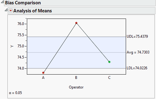
Looking at the Bias Comparison chart, you make the following observations:
• Operator A and Operator B have detectable measurement bias, as they are significantly different from the overall average.
• Operator A is significantly biased low.
• Operator B is significantly biased high.
• Operator C is not significantly different from the overall average.
Classify Your Measurement System
Examine the EMP Results report to classify your measurement system and look for opportunities for improvement. Click the red triangle next to Measurement Systems Analysis for Y and select EMP Results.
Figure 4.12 EMP Results
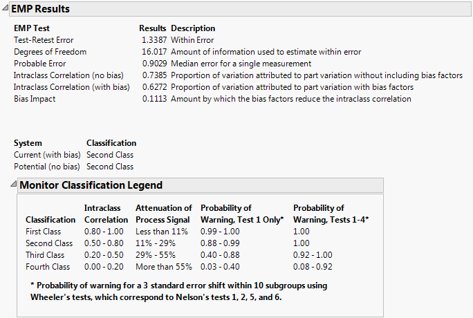
The classification is Second Class, which means that there is a better than 88% chance of detecting a three standard error shift within ten subgroups, using Test one only. You notice that the bias factors have an 11% impact on the Intraclass Correlation. In other words, if you could eliminate the bias factors, your Intraclass Correlation coefficient would improve by 11%.
Explore the Ability of a Control Chart to Detect Process Changes
Use the Shift Detection Profiler to explore the probability that a control chart will be able to detect a change in your process. Click the red triangle next to Measurement Systems Analysis for Y and select Shift Detection Profiler.
Figure 4.13 Shift Detection Profiler
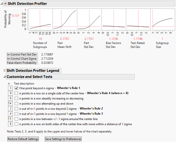
By default, the only test selected is for a point beyond the 3 sigma limits. Also note that the default Subgroup Size is 1, indicating that you are using an Individual Measurement chart.
Explore your ability to detect a shift in the mean of two part standard deviations in the 10 subgroups following the shift. Click the Part Mean Shift value of 2.1701 and change it to 4.34 (2.17 multiplied by 2). The probability of detecting a shift of twice the part standard deviation is 56.9%.
Next, see how eliminating bias affects your ability to detect the shift of two part standard deviations. Change the Bias Factors Std Dev value from 1.1256 to 0. The probability of detecting the shift increases to 67.8%.
Finally, add more tests to see how your ability to detect the two part standard deviation shift changes. In addition to the first test, select the second, fifth, and sixth tests (Wheeler’s Rules 4, 2, and 3). With these four tests and no bias variation, your probability of detecting the shift is 99.9%.
You can also explore the effect of using a control chart based on larger subgroup sizes. For subgroup sizes of two or more, the control chart is an XBar-chart. Change the Bias Factors Std Dev value back to 1.1256 and deselect all but the first test. Set the Subgroup Size in the profiler to 4. The probability of detecting the two part standard deviation shift is 98.5%.
Examine Measurement Increments
Finally, see how well your measurement increments are working. Click the red triangle next to Measurement Systems Analysis for Y and select Effective Resolution.
Figure 4.14 Effective Resolution
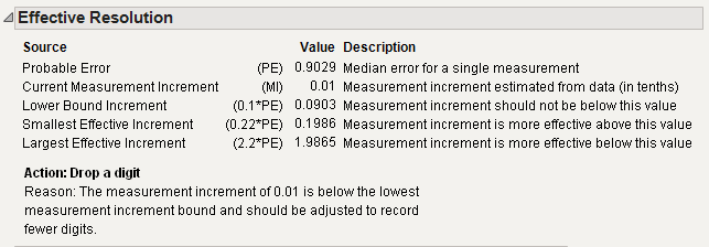
The Current Measurement Increment of 0.01 is below the Lower Bound Increment of 0.09, indicating that you should adjust your future measurements to record one less digit.