 Additional Example of Structural Equation Models
In this example, you are building the structural equation model for industrialization and political democracy described in Bollen (1989), which uses data from 75 developing countries. The variables in the data table include four measures of democracy in 1960 and 1965, and three measures of industrialization in 1960. These variables are described in the Notes column property in each column of the data table. To view the Notes column property, right-click a column name, select Column Info, and select Notes under Column Properties. The type of structural equation model you are building is a structural regression model.
There are four main steps to the model specification process: creating latent variables, adding the loading and regression variables, adding the covariance terms, and placing constraints on the loading variables.
1. Select Help > Sample Data Library and open Political Democracy.jmp.
2. Select Analyze > Multivariate Methods > Structural Equation Models.
3. Select Prod60 through Legis65 and click Model Variables.
4. Click OK.
The Structural Equation Models report Model Specification outline appears.
5. Click the Lists tab in the View panel box.
Create Latent Variables
6. Select Prod60 through Labor60 in the To List, type Ind60 in the box next to Add Latent, and click Add Latent.
7. Select FrPress60 through Legis60 in the To List, type Dem60 in the box next to Add Latent, and click Add Latent.
8. Select FrPress65 through Legis65 in the To List, type Dem65 in the box next to Add Latent, and click Add Latent.
Add Loading and Regression Variables
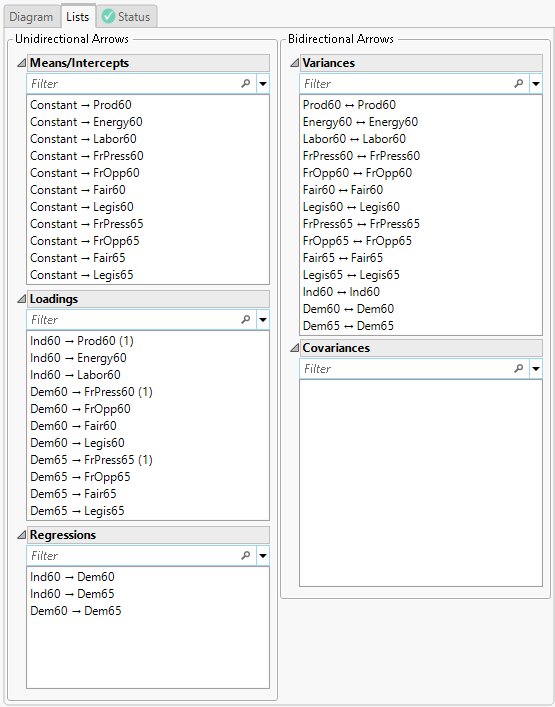
9. Select Ind60 in the From List, select Dem60 in the To List, and click the unidirectional arrow  button.
10. Select Ind60 in the From List, select Dem65 in the To List, and click the unidirectional arrow button.
11. Select Dem60 in the From List, select Dem65 in the To List, and click the unidirectional arrow button.
Figure 8.7 Loadings and Regressions
Add Covariances
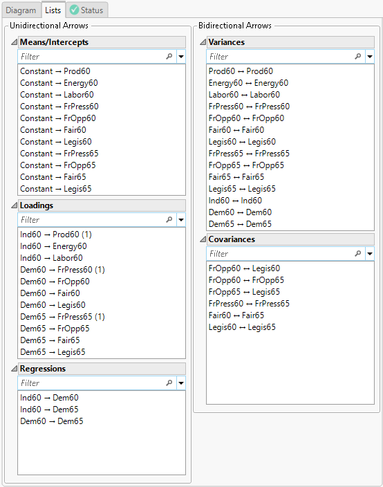
12. Select FrOpp60 in the From List, select Legis60 and FrOpp65 in the To List, and click the bidirectional arrow  button.
13. Select FrOpp65 in the From List, select Legis65 in the To List, and click the bidirectional arrow button.
14. Select FrPress60 in the From List, select FrPress65 in the To List, and click the bidirectional arrow button.
15. Select Fair60 in the From List, select Fair65 in the To List, and click the bidirectional arrow button.
16. Select Legis60 in the From List, select Legis65 in the To List, and click the bidirectional arrow button.
Figure 8.8 Covariances
Add Constraints on Loadings
17. Select Dem60->FrOpp60 and Dem65->FrOpp65 in the Loadings list and click Set Equal.
18. Select Dem60->Fair60 and Dem65->Fair65 in the Loadings list and click Set Equal.
19. Select Dem60->Legis60 and Dem65->Legis65 in the Loadings list and click Set Equal.
Figure 8.9 Completed Model Specification
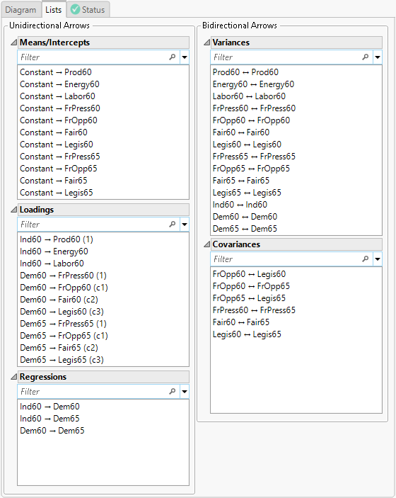
The constraints on the loadings are designated by alphanumeric labels. For example, you can see that Dem60->FrOpp60 and Dem65->FrOpp65 are set equal because they both are labeled “c1”.
20. In the text box below Model Name, type Industrialization and Political Democracy.
21. Click Run.
Figure 8.10 Structural Equation Model Summary of Fit Report
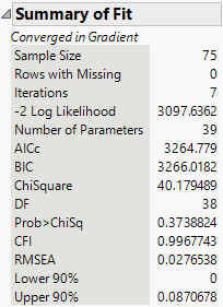
The chi-square statistic for this model, which is listed in the Summary of Fit report, is 40.18 with 38 degrees of freedom. Note that the corresponding p-value is 0.3739, which is not significant. This indicates that there is not evidence to reject the null hypothesis that the model fits well. Therefore, you conclude that this model fits the data reasonably well.
The chi-square value depends on the sample size, and thus, some well-fitting models can still produce a significant chi-square value. The comparative fit index (CFI) and root mean square error of approximation (RMSEA) provide additional guidance for determining model fit. These indices are bounded between 0 and 1. CFI values greater than 0.90 and RMSEA values less than 0.10 are preferred (Browne and Cudeck 1993; Hu and Bentler 1999). Here, the CFI of 0.9968 and RMSEA of 0.0277 indicate a very good fit.
Figure 8.11 Structural Equation Model Parameter Estimates Report
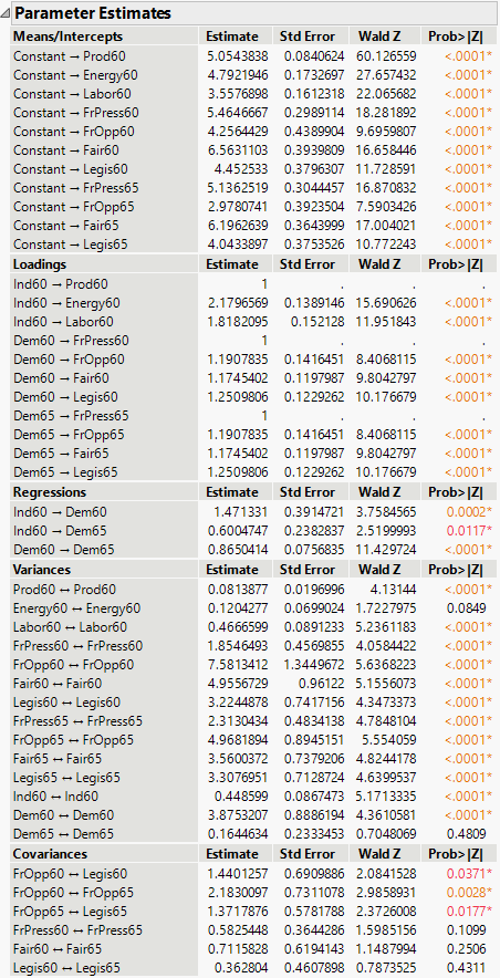
Next, the parameter estimates under Regressions suggest positive effects of Ind60 on Dem60 and Dem65, as well as a positive effect of Dem60 on Dem65. Thus, higher scores on Ind60 are associated with higher Dem60 and Dem65, and higher scores in Dem60 are associated with higher scores in Dem65. The corresponding p-values for the parameter estimates are shown under Regressions. All 3 regression parameters are significant at the α = 0.05 level. Therefore, you conclude that those regression relationships are strong.