Statistical Details for Smoothing Models
Smoothing models are defined as follows:
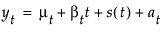
where
μt is the time-varying mean term
βt is the time-varying slope term
s(t) is one of the s time-varying seasonal terms
at are the random shocks
Models without a trend have βt = 0 and nonseasonal models have s(t) = 0. The estimators for these time-varying terms are defined as follows:
Lt is a smoothed level that estimates μt
Tt is a smoothed trend that estimates βt
St - j for j = 0, 1,..., s - 1 are the estimates of the s(t)
Each smoothing model defines a set of recursive smoothing equations that describe the evolution of these estimators. The smoothing equations are written in terms of model parameters called smoothing weights:
α is the level smoothing weight
γ is the trend smoothing weight
ϕ is the trend damping weight
δ is the seasonal smoothing weight
While these parameters enter each model in a different way (or not at all), they have the common property that larger weights give more influence to recent data while smaller weights give less influence to recent data.
Simple Exponential Smoothing
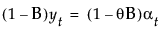
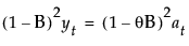
The model for simple exponential smoothing is yt = μt + αt.
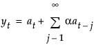
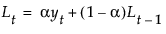
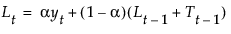
The smoothing equation, Lt = αyt + (1 – α)Lt-1, is defined in terms of a single smoothing weight α. This model is equivalent to an ARIMA(0, 1, 1) model where the following is true:
 where
where 
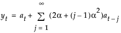
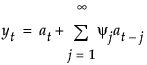
The moving average form of the model is defined as follows:
Double (Brown) Exponential Smoothing
The model for double exponential smoothing is yt = μt + β1t + at.
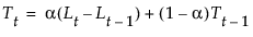
The smoothing equations, defined in terms of a single smoothing weight α, are defined as follows:
This model is equivalent to an ARIMA(0, 1, 1)(0, 1, 1)1 model where the following is true:
 where
where  with
with 
The moving average form of the model is defined as follows:
Linear (Holt) Exponential Smoothing
The model for linear exponential smoothing is yt = μt + βtt + at.
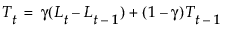
The smoothing equations, in terms of smoothing weights α and γ, are defined as follows:

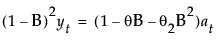
This model is equivalent to an ARIMA(0, 2, 2) model where the following is true:
 with
with  and
and 
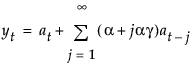
The moving average form of the model is defined as follows:
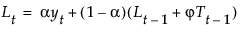
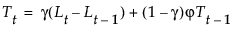
Damped-Trend Linear Exponential Smoothing
The model for damped-trend linear exponential smoothing is yt = μt + βtt + at.
The smoothing equations, in terms of smoothing weights α, γ, and ϕ, are defined as follows:
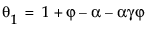
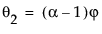
This model is equivalent to an ARIMA(1, 1, 2) model where the following is true:

where
The moving average form of the model is defined as follows:

Seasonal Exponential Smoothing
The model for seasonal exponential smoothing is yt = μt + s(t) + at.
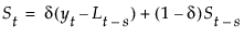
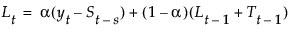
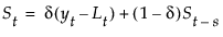
The smoothing equations in terms of smoothing weights α and δ are defined as follows:

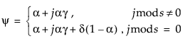
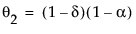
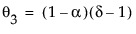
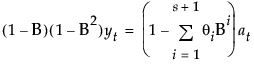
This model is equivalent to a seasonal ARIMA(0, 1, s+1)(0, 1, 0)s model:
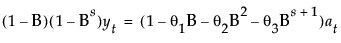
where

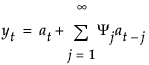
The moving average form of the model is defined as follows:
 where
where 
Winters Method (Additive)
The model for the additive version of the Winters method is yt = μt + βtt + s(t) + at.
The smoothing equations in terms of weights α, γ, and δ are defined as follows:
This model is equivalent to a seasonal ARIMA(0, 1, s+1)(0, 1, 0)s model defined as follows:
The moving average form of the model is defined as follows:
where