Fitting Simple Survival Distributions Using the Nonlinear Platform
The following examples show how to use maximum likelihood methods to estimate distributions from time-censored data when there are no effects other than the censor status.
The Loss Function Templates folder has templates with formulas for exponential, extreme value, loglogistic, lognormal, normal, and one-and two-parameter Weibull loss functions. To use these loss functions, copy your time and censor values into the Time and censor columns of the loss function template. To run the model, select Nonlinear and assign the loss column as the Loss variable. Because both the response model and the censor status are included in the loss function and there are no other effects, you do not need a prediction column (model variable).
Exponential, Weibull, and Extreme-Value Loss Function
The Fan.jmp data table can be used to illustrate the Exponential, Weibull, and Extreme value loss functions discussed in Nelson (1982). The data are from a study of 70 diesel fans that accumulated a total of 344,440 hours in service. The fans were placed in service at different times. The response is failure time of the fans or run time, if censored.
Tip: To view the formulas for the loss functions, in the Fan.jmp data table, right-click the Exponential, Weibull, and Extreme value columns and select Formula.
1. Select Help > Sample Data Library and open Reliability/Fan.jmp.
2. Select Analyze > Specialized Modeling > Nonlinear.
3. Select Exponential and click Loss.
4. Click OK.
5. Make sure that the Loss is Neg LogLikelihood check box is selected.
6. Click Go.
7. Click Confidence Limits.
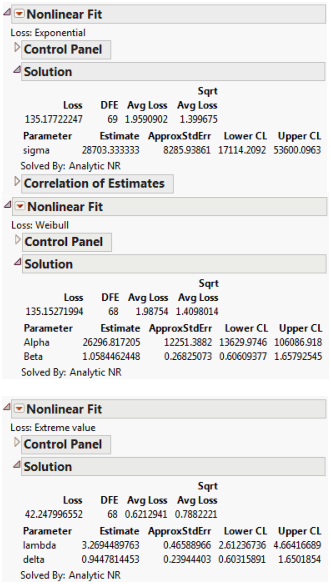
8. Repeat these steps, but select Weibull and Extreme value instead of Exponential.
Figure 14.19 Nonlinear Fit Results
Lognormal Loss Function
The Locomotive.jmp data can be used to illustrate a lognormal loss. The lognormal distribution is useful when the range of the data is several powers of e.
Tip: To view the formula for the loss function, in the Locomotive.jmp data table, right-click the logNormal column and select Formula.
The lognormal loss function can be very sensitive to starting values for its parameters. Because the lognormal distribution is similar to the normal distribution, you can create a new variable that is the natural log of Time and use Distribution to find the mean and standard deviation of this column. Then, use those values as starting values for the Nonlinear platform. In this example, the mean of the natural log of Time is 4.72 and the standard deviation is 0.35.
1. Select Help > Sample Data Library and open Reliability/Locomotive.jmp.
2. Select Analyze > Specialized Modeling > Nonlinear.
3. Select logNormal and click Loss.
4. Click OK.
5. Type 4.72 in the box next to Mu.
6. Type 0.35 in the box next to sigma.
7. Click Go.
8. Click Confidence Limits.
Figure 14.20 Solution Report
The maximum likelihood estimates of the lognormal parameters are 5.11692 for Mu and 0.7055 for Sigma. The corresponding estimate of the median of the lognormal distribution is the antilog of 5.11692, (e5.11692), which is approximately 167. This represents the typical life for a locomotive engine.