Likelihood, AICc, and BIC
Many statistical models in JMP are fit using a technique called maximum likelihood. This technique seeks to estimate the parameters of a model, which we denote generically by β, by maximizing the likelihood function. The likelihood function, denoted L(β), is the product of the probability density functions (or probability mass functions for discrete distributions) evaluated at the observed data values. Given the observed data, maximum likelihood estimation seeks to find values for the parameters, β, that maximize L(β).
Rather than maximize the likelihood function L(β), it is more convenient to work with the negative of the natural logarithm of the likelihood function, -Log L(β). The problem of maximizing L(β) is reformulated as a minimization problem where you seek to minimize the negative log-likelihood (-LogLikelihood = -Log L(β)). Therefore, smaller values of the negative log-likelihood or twice the negative log-likelihood (-2LogLikelihood) indicate better model fits.
You can use the value of negative log-likelihood to choose between models and to conduct custom hypothesis tests that compare models fit using different platforms in JMP. This is done through the use of likelihood ratio tests. One reason that -2LogLikelihood is reported in many JMP platforms is that the distribution of the difference between the full and reduced model -2LogLikelihood values is asymptotically Chi-square. The degrees of freedom associated with this likelihood ratio test are equal to the difference between the numbers of parameters in the two models (Wilks 1938).
The corrected Akaike's Information Criterion (AICc) and the Bayesian Information Criterion (BIC) are information-based criteria that assess model fit. Both are based on -2LogLikelihood.
AICc is defined as follows:

where k is the number of estimated parameters in the model and n is the number of observations used in the model. This value can be used to compare various models for the same data set to determine the best-fitting model. The model having the smallest value, as discussed in Akaike (1974), is usually the preferred model.
BIC is defined as follows:
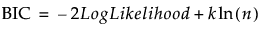
where k is the number of estimated parameters in the model and n is the number of observations used in the model. When comparing the BIC values for two models, the model with the smaller BIC value is considered better.
In general, BIC penalizes models with more parameters more than AICc does. For this reason, it leads to choosing more parsimonious models, that is, models with fewer parameters, than does AICc. For a detailed comparison of AICc and BIC, see Burnham and Anderson (2004).
Simplified Formulas for AICc and BIC in Least Squares Regression
In the case of least squares regression, the AICc and BIC can also be calculated based on the sum of squared errors (SSE). In terms of SSE, AICc and BIC are defined as follows:
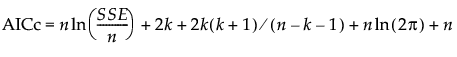
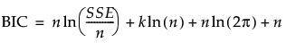
where k is the number of estimated parameters in the model, n is the number of observations used in the model, and SSE is the error sum of squares in the model.