Power for a Single Parameter
This section describes how power for the test of a single parameter is computed. Use the following notation:
X
The model matrix. See Coding for Nominal Effects in Fitting Linear Models for information on the coding for nominal effects. Also, See Model Matrix in the Custom Designs section.
Note: You can view the model matrix by running Fit Model. Then select Save Columns > Save Coding Table from the red triangle menu for the main report.
βι
The parameter corresponding to the term of interest.

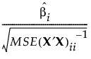
The least squares estimator of βi

The Anticipated Coefficient value. The difference you want to detect is  .
.
The variance of  is given by the ith diagonal entry of
  , where σ2 is the error variance. Denote the ith diagonal entry of
  by
by  .
.
The error variance, σ2, is estimated by the MSE, and has n − p − 1 degrees of freedom, where n is the number of observations and p is the number of terms other than the intercept in the model. If n − p − 1 = 0, then JMP sets the degrees of freedom for the error to 1. This allows the power to be estimated for parameters in a saturated design.
The test of  is given by:
or equivalently by:
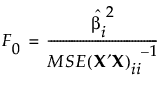
Under the null hypothesis, the test statistic F0 has an F distribution on 1 and n − p − 1 degrees of freedom.
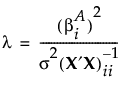
If the true value of  is
is  , then F0 has a noncentral F distribution with noncentrality parameter given by:
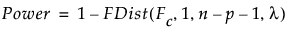
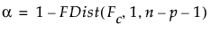
To compute the power of the test, first solve for the α-level critical value Fc:
Then calculate the power as follows: