Prediction Profiler Options
The red triangle menu on the Prediction Profiler title bar has the following options:
Optimization and Desirability
Submenu that consists of the following options:
Desirability Functions
Shows or hides the desirability functions. Desirability is discussed in Desirability Profiling and Optimization.
Maximize Desirability
Sets the current factor values to maximize the desirability functions. Takes into account the response importance weights.
Note: In many situations, the settings that optimize the desirability function are not unique. The Maximize Desirability option gives one such setting. The Contour Profiler is a good tool for finding alternative factor combinations that optimize desirability. For an example, see Explore Optimal Settings in the Contour Profiler section.
Note: If a factor has a Design Role column property value of Discrete Numeric, it is treated as continuous in the optimization of the desirability function. To account for the fact that the factor can assume only discrete levels, it is displayed in the profiler as a categorical term and an optimal allowable level is selected.
Maximize and Remember
Maximizes the desirability functions and remembers the associated settings.
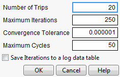
Maximization Options
Opens the Maximization Options window where you can refine the optimization settings.
Figure 3.5 Maximization Options Window
Maximize for Each Grid Point
Used only if one or more factors are locked. The ranges of the locked factors are divided into a grid, and the desirability is maximized at each grid point. This is useful if the model that you are profiling has categorical factors. Then the optimal condition can be found for each combination of the categorical factors.
Save Desirabilities
Saves the three desirability function settings for each response, and the associated desirability values, as a Response Limits column property in the data table. These correspond to the coordinates of the handles in the desirability plots.
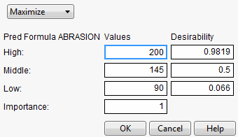
Set Desirabilities
Opens the Response Goal window where you can set specific desirability values.
Figure 3.6 Response Goal Window
Save Desirability Formula
Creates a column in the data table with a formula for Desirability. The formula uses the fitting formula when it can, or the response variables when it cannot access the fitting formula.
Assess Variable Importance
Provides different approaches to calculating indices that measure the importance of factors to the model. These indices are independent of the model type and fitting method. See Assess Variable Importance.
Bagging
(Available only when the Prediction Profiler is embedded in certain modeling platforms.) Launches the Bagging window. Bootstrap aggregating (bagging) enables you to create multiple training data sets by sampling with replacement from the original data. For each training set, a model is fit using the analysis platform, and predictions are made. The final prediction is a combination of the results from all of the models. This improves prediction performance by reducing the error from variance. See Bagging.
Simulator
Launches the Simulator. The Simulator enables you to create Monte Carlo simulations using random noise added to factors and predictions for the model. A typical use is to set fixed factors at their optimal settings, and uncontrolled factors and model noise to random values. You then find out the rate of responses outside the specification limits. See Simulator.
Interaction Profiler
Shows or hides interaction plots that update as you update the factor values in the Prediction Profiler. Use this option to help visualize third degree interactions by seeing how the plot changes as current values for the factors change. The cells that change for a given factor are the cells that do not involve that factor directly.
Confidence Intervals
Shows or hides confidence intervals in the Prediction Profiler plot. The intervals are drawn by bars for categorical factors, and curves for continuous factors. These are available when the profiler is used inside certain fitting platforms or when a standard error column has been specified in the Prediction Profiler launch dialog.
Prop of Error Bars
(Appears when a Sigma column property exists in any of the factor and response variables.) This option displays the 3σ interval that is implied on the response due to the variation in the factor. Propagation of error (POE) is important when attributing the variation of the response in terms of variation in the factor values when the factor values are not very controllable. See Propagation of Error Bars.
Sensitivity Indicator
Shows or hides a purple triangle whose height and direction correspond to the value of the partial derivative of the profile function at its current value. This is useful in large profiles to be able to quickly spot the sensitive cells.
Figure 3.7 Sensitivity Indicators
Profile at Boundary
When analyzing a mixture design, JMP constrains the ranges of the factors so that settings outside the mixture constraints are not possible. This is why, in some mixture designs, the profile traces turn abruptly.
When there are mixture components that have constraints, other than the usual zero-to-one constraint, a new submenu, called Profile at Boundary, appears on the Prediction Profiler red triangle menu. It has the following two options:
Turn At Boundaries
Lets the settings continue along the boundary of the restraint condition.
Stop At Boundaries
Truncates the prediction traces to the region where strict proportionality is maintained.
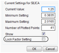
Reset Factor Grid
Displays a window for each factor enabling you to enter a specific value for the factor’s current setting, to lock that setting, and to control aspects of the grid. See the section Set or Lock Factor Values.
Figure 3.8 Factor Settings Window
Factor Settings
Submenu that consists of the following options:
Remember Settings
Adds an outline node to the report that accumulates the values of the current settings each time the Remember Settings command is invoked. Each remembered setting is preceded by a radio button that is used to reset to those settings. There are options to remove selected settings or all settings in the Remember Settings red triangle menu.
Set To Data in Row
Assigns the values of a data table row to the X variables in the Prediction Profiler.
Copy Settings Script
Copies the current Prediction Profiler’s settings to the clipboard.
Paste Settings Script
Pastes the Prediction Profiler settings from the clipboard to a Prediction Profiler in another report.
Append Settings to Table
Appends the current profiler’s settings to the end of the data table. This is useful if you have a combination of settings in the Prediction Profiler that you want to add to an experiment in order to do another run.
Broadcast Factor Settings
Sends the current profiler’s factor settings to all other profilers, but does not link the profilers. A change in a factor in one profiler does not cause changes in any other profilers unless Broadcast Factor Settings is selected again.
Link Profilers
Links all the profilers together. A change in a factor in one profiler causes that factor to change to that value in all other profilers, including Surface Plot. This is a global option, set, or unset for all profilers.
Set Script
Sets a script that is called each time a factor changes. The set script receives a list of arguments of the form:
{factor1 = n1, factor2 = n2, ...}For example, to write this list to the log, first define a function:
ProfileCallbackLog = Function({arg},show(arg));Then enter ProfileCallbackLog in the Set Script dialog.
Similar functions convert the factor values to global values:
ProfileCallbackAssign = Function({arg},evalList(arg));Or access the values one at a time:
ProfileCallbackAccess = Function({arg},f1=arg["factor1"];f2=arg["factor2"]);Unthreaded
Enables you to change to an unthreaded analysis if multithreading does not work.
Default N Levels
Enables you to set the default number of levels for each continuous factor. This option is useful when the Prediction Profiler is especially large. When calculating the traces for the first time, JMP measures how long it takes. If this time is greater than three seconds, you are alerted that decreasing the Default N Levels speeds up the calculations.
Output Grid Table
Produces a new data table with columns for the factors that contain grid values, columns for each of the responses with computed values at each grid point, and the desirability computation at each grid point.
If you have a lot of factors, it is impractical to use the Output Grid Table command, because it produces a large table. A memory allocation message might be displayed for large grid tables. In such cases, you should lock some of the factors, which are held at locked, constant values. To get the window to specify locked columns, ALT- or Option-click inside the profiler graph to get a window that has a Lock Factor Setting check box.
Output Random Table
Prompts for a number of runs and creates an output table with that many rows, with random factor settings and predicted values over those settings. This is equivalent to (but much simpler than) opening the Simulator, resetting all the factors to a random uniform distribution, then simulating output. This command is similar to Output Grid Table, except it results in a random table rather than a sequenced one.
The prime reason to make uniform random factor tables is to explore the factor space in a multivariate way using graphical queries. This technique is called Filtered Monte Carlo.
Suppose you want to see the locus of all factor settings that produce a given range to desirable response settings. By selecting and hiding the points that do not qualify (using graphical brushing or the Data Filter), you see the possibilities of what is left: the opportunity space yielding the result that you want.
Some rows might appear selected and marked with a red dot. These represent the points on the multivariate desirability Pareto Frontier - the points that are not dominated by other points with respect to the desirability of all the factors.
Alter Linear Constraints
Enables you to add, change, or delete linear constraints. The constraints are incorporated into the operation of Prediction Profiler. See Linear Constraints.
Save Linear Constraints
Enables you to save existing linear constraints to a table script called Constraint. See Linear Constraints.
Conditional Predictions
Appears when random effects are included in the model. The random effects predictions are used in formulating the predicted value and profiles.
Appearance
Submenu that consists of the following options:
Arrange in Rows
Enter the number of plots that appear in a row. This option helps you view plots vertically rather than in one wide row.
Reorder X Variables
Opens a window where you can reorder the model main effects by dragging them to the desired order.
Reorder Y Variables
Opens a window where you can reorder the responses by dragging them to the desired order.
Adapt Y Axis
Re-scales the vertical axis if the response is outside the axis range, so that the range of the response is included.
Show Creator
Shows or hides the name of the platform that created the formula in the response column. The platform name appears on the vertical axis. (Available only if the response column contains a “Creator” named argument in the “Predicting” column property.)