Statistical Details for the Reliability Demonstration Calculator

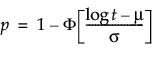
The reliability demonstration depends on the assumed failure time distribution with scale parameter σ. The reliability standard, or probability of survival at time t and location μ is stated as follows:

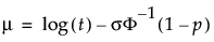
where μ is solved for using the following:

To calculate sample size and the size of the test, the probability of survival at time t is posed as a hypothesis test:

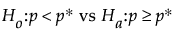
where p* is the standard probability of survival at time t*.

We want to test the hypothesis at the α level or as follows:

α = Pr(k or few failures | H0 true).

Since the test is of n independent units, the number of failures has a binomial (n, p) distribution where p is the probability of a unit failing before time t. Therefore, we can express α as a function of t and n:

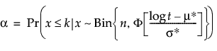
where μ* and σ* are from the assumed reliability standard.

Properties of the binomial and beta distributions result in being able to solve for t using:

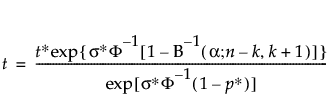
For n, Brent’s method is used to find the root of:

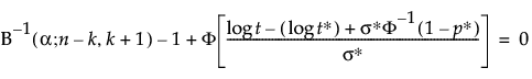
where:

B−1(α; n − k, k + 1) is the α quantile of the Beta(n − k; k + 1) distribution

and Φ() is the cumulative distribution function of the assumed failure time distribution.

For more information about calculations in JMP, see Barker (2011, Section 5).