Example of a Generalized Linear Model
This example uses Poisson regression to model count data from a study of nesting horseshoe crabs. Each female crab had a male crab resident in her nest. The study investigated whether there were other males, called satellites, residing nearby. The data table CrabSatellites.jmp contains a response variable listing the number of male satellites, as well as variables that describe the color, spine condition, weight, and carapace width of the female crab. You are interested in the relationship between the number of satellites and the variables that describe the female crabs.
To fit the Poisson regression model, follow these steps:
1. Select Help > Sample Data Library and open CrabSatellites.jmp.
2. Select Analyze > Fit Model.
3. Select satell and click Y.
4. Select color, spine, width, and weight and click Add.
5. From the Personality list, select Generalized Linear Model.
6. From the Distribution list, select Poisson.
In the Link Function list, Log should be selected for you automatically.
7. Click Run.
Figure 12.2 Crab Satellite Results
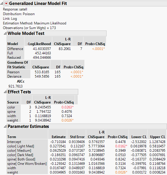
The Whole Model Test shows that the difference between log-likelihoods for the full and reduced models is 41.6. The Prob>ChiSq value is equivalent to the p-value for a whole model F test. A p-value less than 0.0001 indicates that the model as a whole is significant. The report also contains the corrected Akaike Information Criterion (AICc), 921.7613. This value can be compared with other models to determine the best-fitting model for the data. Smaller AICc values indicate better fitting models.
The Effects Tests report shows that weight is a significant factor in the model. Note that the p-value for weight, 0.0026, is the same in the Parameter Estimates table as well, since weight is a continuous variable.
The Effect Tests report also shows that the categorical variable color is significant. Color has four levels, Light Med, Medium, Dark Med, and Dark. The parameter estimates for the first three levels are shown in the Parameter Estimates table. The parameter estimate for Dark is the negative of the sum of the parameter estimates for the first three levels.
You can use the Prediction Profiler to further explore the model.
8. Click the red triangle next to Generalized Linear Model Fit and select Profilers > Profiler.
Figure 12.3 Prediction Profiler for Satell
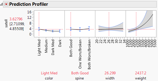
The confidence band on weight indicates that there is less variability in the model for smaller weight values than there is for larger weight values. The profiler enables you to easily explore the levels of the categorical variables. From the profiler, you can see that the predicted number of satellite crabs decreases as the color of the crab changes from light to dark.