Example of the Simulator
Use sequencing to examine how the distribution of the response changes when the mean (sequencing location) and variability (sequencing spread) of the inputs change.
1. Select Help > Sample Data Library and open Tiretread.jmp.
2. Select Graph > Profiler.
3. Select Pred Formula ABRASION and Pred Formula MODULUS and click Y, Prediction Formula.
4. Click OK.
5. Click the Prediction Profiler red triangle and select Simulator.
6. Beneath each factor select Random.
Note: The default random distribution is a normal distribution.
7. Change the N Runs value to 1000.
8. Open Simulate to Table outline and then open the Sequencing outline.
Figure 8.2 Simulator Settings
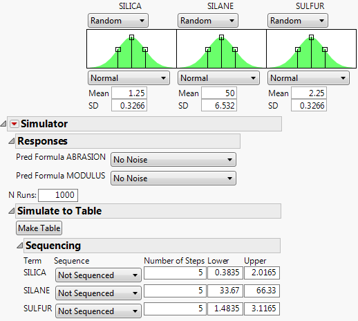
You want to examine how the responses change as the input factors change locations. To explore changes in factor mean, use sequence location. To instead explore changes in the variability of the factor, use sequence spread.
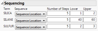
9. For SILICA, select Sequence Location. Leave the number of steps set to 5. Set the Lower limit to 1 and the Upper limit to 2.
10. For SILANE, select Sequence Location. Leave the number of steps set to 5. Set the Lower limit to 40 and the Upper limit to 60.
11. For SULFUR, select Sequence Location. Leave the number of steps set to 5. Set the values Lower limit to 2 and the Upper limit to 3.
Figure 8.3 Sequencing Settings
12. Click Make Table.
The SILICA Mean, SILANE Mean, and SULFUR Mean columns contain five steps across their respective range of values. For example, the Silica Mean values are 1, 1.25, 1.5, 1.75, and 2. The SILICA, SILANE, and SULFUR columns are the simulated values from a normal distribution with a mean defined by the corresponding mean columns and a fixed standard deviation. Pred Formula ABRASION and Pred Formula MODULUS values are calculated for set of simulated values, so that you can explore how the responses change as the factor values change.
13. Select Analyze > Distribution.
14. Select SILICA Mean and Pred Formula ABRASION and click Y, Columns.
15. Click OK.
Figure 8.4 Distribution of SILICA Mean by Pred Formula ABRASION
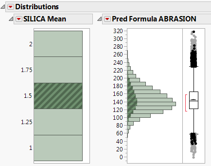
Click a histogram bar that corresponds to a SILICA Mean to see how the predicted value for abrasion varies across the simulated silane and sulfur ranges given the selected value of silica.