Examples of the One Sample Mean Calculator
In the following examples, suppose you are interested in demonstrating that the flammability of a new fabric being developed by your company has improved performance over current materials. Previous testing indicates that the standard deviation for time to burn of this fabric is 2 seconds.
Example of Sample Size Calculation
In this initial example, you would like to design an experiment that has 90% power to detect a difference of 1.5 seconds at a significance level of α = 0.05. Use the One Sample Mean calculator to calculate the number of fabric samples you need to test.
1. Select DOE > Design Diagnostics > Sample Size and Power.
2. Click the One Sample Mean button.
3. Leave Alpha set to 0.05.
4. Enter 2 for Std Dev.
5. Leave Extra Parameters set to 0.
6. Enter 1.5 for Difference to detect.
7. Leave Sample Size blank.
8. Enter 0.9 for Power.
9. Click Continue.
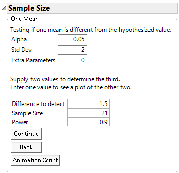
Figure 17.4 One-Sample Mean Calculator
At a significance level of 0.05, 21 fabric samples are needed to have a 90% chance of detecting a significant difference of 1.5 seconds in the burn time.
Example of Power versus Sample Size Plot
To explore trade offs between sample size and power in your fabric experiment, use the plot of power versus sample size.
1. Select DOE > Design Diagnostics > Sample Size and Power.
2. Click One Sample Mean.
3. Leave Alpha set to 0.05.
4. Enter 2 for Std Dev.
5. Leave Extra Parameters set to 0.
6. Enter 1.5 for the Difference to detect.
7. Leave Sample Size blank.
8. Leave Power blank.
9. Click Continue to launch the power by sample size plot.
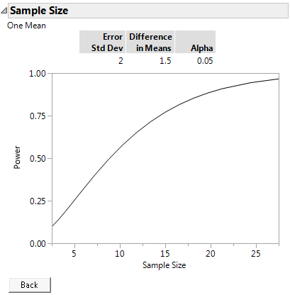
Figure 17.5 Power by Sample Size
The plot shows a range of sample sizes for which the power varies from about 0.1 to about 0.95. You could reduce the number of tests in your experiment to about 15 and maintain power above 75%. However, if you ran only 10 tests, the power to detect a significant difference of 1.5 would drop to about 50%.
Tip: Use the crosshair tool to obtain sample size and power combinations from the plot.
Example of Power versus Difference Plot
To explore trade offs between power and the magnitude of the difference that you can detect with 21 observations in your fabric experiment, use the plot of power versus difference.
1. Select DOE > Design Diagnostics > Sample Size and Power.
2. Click One Sample Mean.
3. Leave Alpha set to 0.05.
4. Enter 2 for Std Dev.
5. Leave Extra Parameters set to 0.
6. Leave Difference to detect blank.
7. Enter 21 for Sample Size.
8. Leave Power blank.
9. Click Continue.
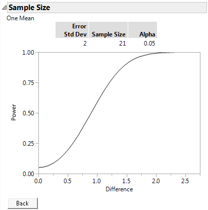
Figure 17.6 Plot of Power by Difference to Detect for a Sample Size of 21
At a significance level of 0.05 and 21 observations, you can detect a difference of 1.5 seconds with 90% power. If the difference is only one second smaller, then with 21 fabric samples, you have about 50% power of detecting the difference.
Example of an Animation Script
Use an animation script to explore how changing the sample size affects power.
1. Select DOE > Design Diagnostics > Sample Size and Power.
2. Click One Sample Mean.
3. Leave Alpha set to 0.05.
Tip: You can change the Alpha level after the animation is launched by clicking the Alpha value in the animation window.
4. Enter 2 for Std Dev.
5. Leave Extra Parameters set to 0.
6. Enter 1.5 as Difference to detect.
7. Leave Sample Size blank.
Tip: When you leave the sample size blank, the default sample size is set to 20. You will see the default of 20 after the animation script is launched. You can change the sample size before or after the animation is launched. To change it after the animation is launched, click the Sample Size value in the animation window.
8. Leave Power blank.
9. Click Animation Script.
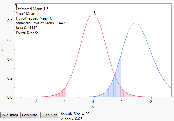
Figure 17.7 Initial Animation Script to Illustrate Power
The initial animation plot shows two t-density curves:
– The red curve shows the t-distribution when the true mean is zero.
– The blue curve shows the t-distribution when the true mean is 1.5, which is the difference to be detected.
– The blue shading indicates the probability of committing a type II error. A type II error is the probability of not detecting a difference when there is a difference. The probability of a type II error is often denoted by β.
– The red shading indicates the probability of committing a type I error. A type I error is the probability of concluding that the difference in means is significant when there is no difference. The probability of a type I error is often denoted by α.
Select and drag the square handles to see the changes in statistics based on the positions of the curves. To change the values of Sample Size and Alpha, click their values beneath the plot.
By default, the animation shows a two sided test. Use the Two Sided, Low Side, and High Side buttons to toggle between not equal, less than, or greater than alternative hypotheses.


