Plot Functions
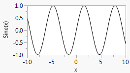
A Y Function() function is used to draw smooth functions. The first argument is the expression to be plotted. The second argument is the name of the X variable in the expression.
win = New Window( "Sine Function",
Graph Box(
Frame Size( 200, 100 ),
X Scale( -10, 10 ),
Y Scale( -1, 1 ),
X Name( "x" ),
Y Name( "Sine(x)" ),
Y Function( Sine( x ), x ) ) );
Figure 12.32 Sine Wave
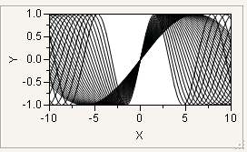
You can use For to overlap several sine waves:
win = New Window( "Overlapping Sine Waves",
Graph Box(Frame Size( 200, 100 ),
X Scale( -10, 10 ),
Y Scale( -1, 1 ),
For( i = 1, i <= 4, i += .1,
Y Function( Sine( x / i ), x )
)
)
);
Figure 12.33 Overlapping Sine Waves
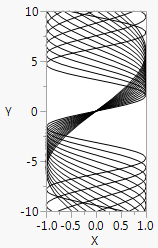
Similarly, X Function() is for drawing a graph where the symbol is varied on the Y variable.
win = New Window( "Overlapping Sine Waves",
Graph Box(Frame Size( 100, 200 ),
X Scale( -1, 1 ),
Y Scale( -10, 10 ),
For( i = 1, i <= 4, i += .2,
X Function( Sine( y / i ), y )
)
)
);
Figure 12.34 Overlapping Sine Waves along the X-Axis
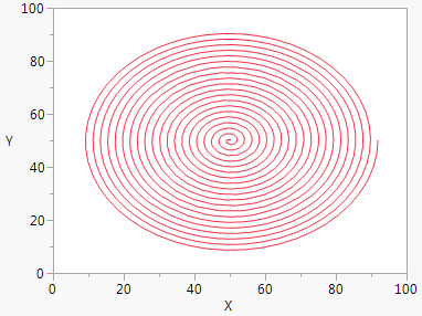
An XY Function() draws a smooth curve using a pair of formulas (parametric equations) that depend on a third variable. The third variable’s value is incremented from a minimum value to a maximum value to generate the X-Y pairs.
win = New Window( "Spiral",
Graph Box(Pen Color( "red" ); // red line color
xCenter = 50; // location of the center of the curve on the x axis
yCenter = 50; // location of the center of the curve on the y axis
minAngle = 0;maxAngle = Pi() * 2 * 20;
XY Function(xCenter + ((ta / 3) * Cos( ta )),
yCenter + ((ta / 3) * Sin( ta )),
ta,
Min( minAngle ), Max( maxAngle ),Inc( Pi() / 100 )
);
)
);
In this example, Sin() and Cos() use ta as an argument (rotates) and as a factor (expands). (Sin() and Cos() use radians, not degrees.)
Figure 12.35 Spiral Parametric Plot
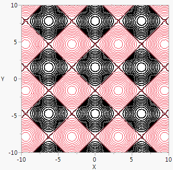
Contour Function() is an analogous way to represent a three-dimensional function in a two-dimensional space. The final argument specifies the value(s) for the contour line(s). The argument can be a value, an indexed range of values using ::, or a matrix of values.
win = New Window( "Bird's eye view of the egg carton function",
Graph Box(Frame Size( 300, 300 ),
X Scale( -10, 10 ),
Y Scale( -10, 10 ),
Pen Color( "black" );
Pen Size( 2 );
Contour Function( Sine( y ) + Cosine( x ), x, y, (0 :: 20) / 5 );
Pen Color( "red" );
Pen Size( 1 );
Contour Function( Sine( y ) + Cosine( x ), x, y, (-20 :: 0) / 5 );
)
);
Figure 12.36 Egg Carton Function
Normal Contour() draws normal probability contours for k populations and two variables. The first argument is a scalar probability or a matrix of probability values for the contours. Subsequent arguments are matrices to specify means, standard deviations, and correlations. The mean and standard deviation matrices have dimension k × 2. The correlation matrix should be k × 1, where the first row pertains to the first contour, the second row to the second contour, and so on. The first column is for x and the second column for y. Consider the following example:
Normal Contour(
[ prob1,
prob2,
prob3, ...],
[ xmean1 ymean1,
xmean2 ymean2,
xmean3 ymean3, ...],
[ xsd1 ysd1,
xsd2 ysd2,
xsd3 ysd3, ...],
[ xycorr1,
xycorr2,
xycorr3, ...]);
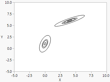
The following script draws contours at probabilities 0.1, 0.5, 0.7, and 0.99 for two populations and two variables. The first population has x mean 0 and y mean 1, with standard deviation 0.3 along the x axis and 0.6 along the y-axis, and with correlation 0.5. The second has x mean 4 and y mean 6, with standard deviation 0.8 along the x axis and 0.4 along the y-axis, and with correlation 0.9.
win = New Window( "Normal Contours",
Graph Box(X Scale( -5, 10 ),
Y Scale( -5, 10 ),
Normal Contour( [.1, .5, .7, .99], [0 1, 4 6], [.3 .6, .8 .4], [.5, .9] )
)
);
Figure 12.37 Normal Contour Function
Normal Contour() is a general way to accomplish effects such as Bivariate’s density ellipses. The Bivariate script in the Football.jmp sample data creates an example.
Gradient Function
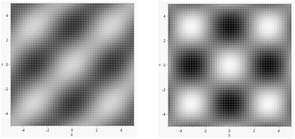
Gradient Function() fills a set of rectangles on a grid according to a color determined by the expression value as it crosses a range corresponding to a range of colors.
Gradient Function( expression, xname, yname, [zlow, zhigh], ZColor( [colorLow, colorHigh] ), <XGrid( min, max, incr )>, <YGrid( min, max, incr )>, <Transparency( t )>;
Here are explanations of the elements in the Gradient Function() syntax:
GradientFunction(/* the expression to be contoured, which is a function in terms of
the two variables that follow expression*/
Expression,
// the two variable names used in the expression
xname, yname,
// the low and high expression values the gradient is scaled between
[zlow, zhigh],
// the colors that correspond to the low value and the high value
ZColor([colorLow, colorHigh])
// optional specification for the grid of values
<XGrid(min, max, incr),>
<YGrid(min, max, incr)> );
/* the value 0 means clear. The value 1 means completely opaque and
is the usual drawing mode. */
<Transparency>
The ZColor() values must be numeric codes rather than names. You can use the color menu indices (such as 0=black, 1=grey, 2=white, 3=red, 4=green, and 5=blue) found in Specify Colors.
The following example uses Gradient Function() to create an animated graph.
phase = 0.7;win = New Window( "Gradient Function",
a = Graph(Frame Size( 400, 400 ),
X Scale( -5, 5 ),
Y Scale( -5, 5 ),
Gradient Function(phase * Sine( x ) * Sine( y ) + (1 - phase) * Cosine( x ) * Cosine( y ),
x,
y,
[-1 1],zcolor( [0, 2] )
)
)
);
b = a[FrameBox( 1 )];For( i = 1, i <= 5, i++,
For( phase = 0, phase < 1, phase += 0.05,
b << Reshow;Wait( 0.01 );
);
For( phase = 1, phase > 0, phase -= 0.05,
b << Reshow;Wait( 0.01 );
);
);
Figure 12.38 Gradient Function
