Box Cox Y Transformation
A Box-Cox power transformation is used to transform the response so that the usual regression assumptions of normality and homogeneity of variance are more closely satisfied. The transformed response can then be fit using a regression model. However, you can also use the Box-Cox power transformation to transform a variable for other reasons. This transformation is appropriate only when the response, Y, is strictly positive.
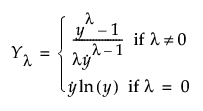
A commonly used transformation raises the response to some power. Box and Cox (1964) formalized and described this family of power transformations. The formula for the transformation is constructed to provide a continuous definition in terms of the parameter λ, and so that the error sums of squares are comparable. Specifically, the following equation provides the family of transformations:

Here,  denotes the geometric mean.
The Box Cox Y Transformation option fits transformations from λ = –2 to 2 in increments of 0.2. To choose a value of λ, the likelihood function for each of these transformations is computed. They are computed under the assumption that the errors are independent and normal with mean zero and variance σ2. The value of λ that maximizes the likelihood is selected. This value also minimizes the SSE over the values of λ. The value of λ that minimizes the SSE is found using a quadratic interpolation between the two incremental grid points surrounding the grid point with the smallest SSE. If this interpolation results in a negative SSE value, then the grid value of λ that minimizes the SSE is reported as the best λ.
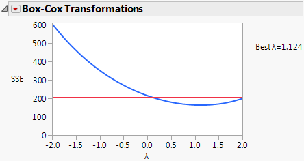
The Box-Cox Transformations report displays a plot showing the sum of squared errors (SSE) values against the values of λ. The horizontal red line on the plot represents a one-sided 95% confidence interval for λ. This confidence interval is based on the confidence region defined in Box and Cox (1964, p. 216). The confidence region is defined by the following inequality:
SSE(λ) < SSE(λbest) * exp(ChiSquareQuantile(0.95,1) / dfe)
where
SSE(λbest) is the SSE calculated using the reported Best λ
ChiSquareQuantile(0.95,1) is the 0.95th quantile of a χ2 distribution with 1 degree of freedom
dfe is the error degrees of freedom in the Analysis of Variance table for the regression model
The Box Cox Transformations report provides the following options:
Refit with Transform
Enables you to specify a value for lambda to define a transformed Y variable and then provides a least squares fit to the transformed variable.
Replace with Transform
Enables you to specify a value for lambda to define a transformed Y variable and then replaces the existing least squares fit with a fit to the transformed variable. If you have multiple responses, Replace with Transform replaces only the report for the response that you are transforming.
Save Best Transformation
Creates a new column in the data table and saves the formula for the best transformation.
Save Specific Transformation
Enables you to specify a value for lambda and creates a column in the data table with the formula for your specified transformation.
Table of Estimates
Creates a new data table containing parameter estimates and SSE values for all λ from –2 to 2, in increments of 0.2.
Example of Box-Cox Y Transformation
1. Select Help > Sample Data Library and open Reactor.jmp.
2. Select Analyze > Fit Model.
3. Select Y and click Y.
4. Make sure that the Degree box has a 2 in it.
5. Select F, Ct, A, T, and Cn and click Macros > Factorial to Degree.
6. Click Run.
7. Click the Response Y red triangle and select Factor Profiling > Box Cox Y Transformation.
Figure 3.53 Box Cox Y Transformation
The plot shows that the best values of λ are between 0.1 and 2.0. The value that JMP selects, using interpolation between the best two values in the 0.2-unit grid of λ values, is 1.124.
8. (Optional) To see the SSE values used to construct the graph, select Table of Estimates.
