Example of Generalized Regression for Wide Data
Wide data is the term used to describe a data set where there are more predictors than there are observations. For wide data, traditional regression methods are not practical. Regression methods that incorporate variable selection enable you to fit a regression model in these situations. In this example, you compare three models with varying degrees of variable selection.
1. Select Help > Sample Data Folder and open Prostate Cancer.jmp.
2. Select Analyze > Fit Model.
3. Select Status from the Select Columns list and click Y.
Because this is a Nominal response column, the Personality changes to Nominal Logistic and the Target Level option appears. The default value for this option is CCD, because that is the value specified in the Target Level column property in the data table.
4. From the Personality list, select Generalized Regression.
The Distribution list automatically shows the Binomial distribution. This is the only distribution available when Y is binary and has a Nominal modeling type.
5. Select the Proteins column group from the Select Columns list and click Add.
This adds all 667 columns in the column group to the model.
6. Click Run.
The Generalized Regression report that appears contains a Model Launch control panel. There is no initial Logistic Regression model fit because the number of predictors is greater than the number of observations.
7. Select Elastic Net as the Estimation Method.
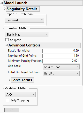
8. Click the gray disclosure icon next to Advanced Controls.
Figure 7.8 Advanced Controls
9. Select Smallest in Green Zone as the Initial Displayed Solution.
10. Click Go.
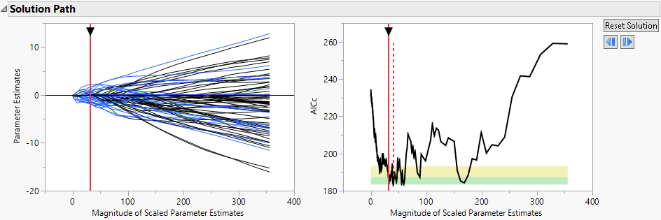
Figure 7.9 Smallest in Green Zone Model
The Solution Path shows the smallest model that is considered comparable to the minimum AICc model, where smallest model means the one with the fewest parameters.
11. Click the gray disclosure icon next to Binomial Elastic Net with AICc Validation.
12. Click the gray disclosure icon next to Model Launch.
13. Select Best Fit as the Initial Displayed Solution.
14. Click Go.
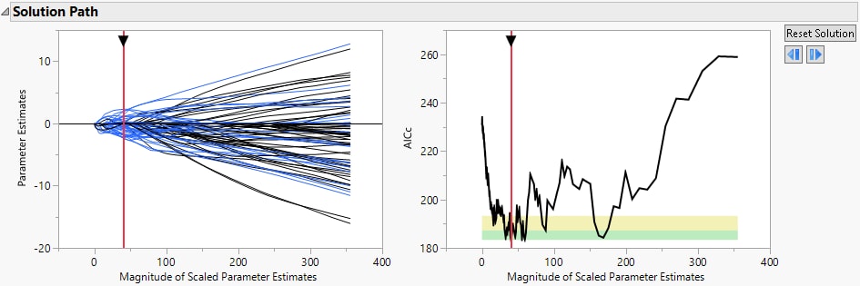
Figure 7.10 Best Fit Model
The Solution Path shows the best fit model, where best fit means the one with the minimum AICc value.
15. Click the gray disclosure icon next to Binomial Elastic Net with AICc Validation.
16. Click the gray disclosure icon next to Model Launch.
17. Select Biggest in Green Zone as the Initial Displayed Solution.
18. Click Go.
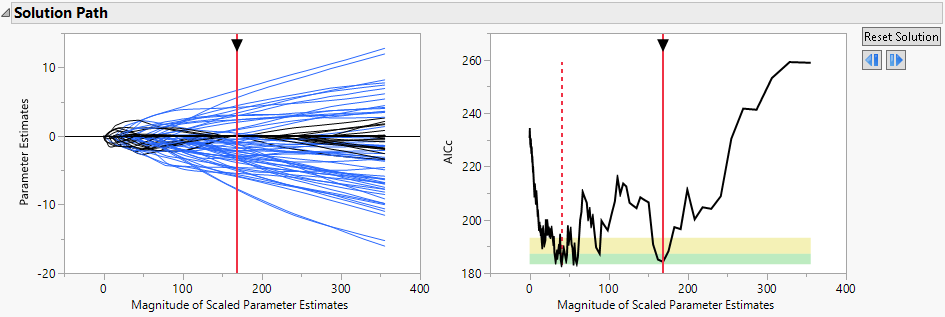
Figure 7.11 Biggest in Green Zone Model
The Solution Path shows the largest model that is considered comparable to the minimum AICc model, where largest model means the one with the most parameters.
19. Click the gray disclosure icon next to Binomial Elastic Net with AICc Validation.
Figure 7.12 Model Comparison Table
The Model Comparison report shows the three models. You can identify the size of each model using the Nonzero Parameters column. As the number of parameters in the models increases, the Generalized RSquare values increase. Because these models are all in the green zone, there is strong evidence that any of these models are comparable to the best model.


