Example of Multiple Correspondence Analysis
In this example, you explore the associations between employee responses to four questions to gain an understanding of different groups of employees. This example uses data collected from 55 JMP employees about their preferences, or tastes, in these areas:
• Preferred TV program (8 categories): news, comedy, police, nature, sport, film, drama, or soap operas.
• Preferred film (8 categories): action, comedy, costume drama, documentary, horror, musical, romance, or SciFi.
• Preferred type of art (7 categories): performance, landscape, renaissance, still life, portrait, modern, or impressionism.
• Preferred place to eat out (6 categories): burgers & fries, pub, Indian restaurant, Italian restaurant, French restaurant, or steak house.
Note: The measures for preferences are based on questions from LeRoux and Rouanet (2010).
1. Select Help > Sample Data Folder and open Employee Taste.jmp.
2. Select Analyze > Multivariate Methods > Multiple Correspondence Analysis.
3. Select TV, Film, Art, and Restaurant and click Y, Response.
In MCA, as in principal component analysis, factors are typically considered responses rather than some being responses and others explanatory.
4. Click OK.
Tip: Click and drag overlapping labels to rearrange them.
5. Below the plot, select Proportional marker size.
The marker size indicates the relative proportion of responses in that category.
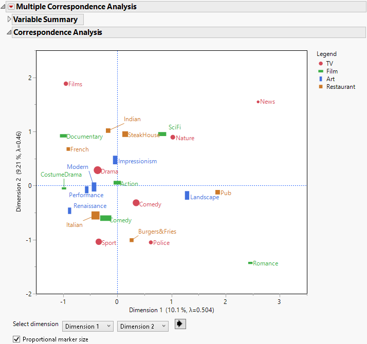
Figure 7.2 Part of the Initial Multiple Correspondence Analysis Report
The Correspondence Analysis report shows the projection of categories of the four variables onto the first two principal axes, or dimensions. Use the controls to change the dimensions plotted. The distance between points represents the dissimilarity between response patterns of the employees.
From this graph, you can use your knowledge of the subject matter to interpret the findings:
– Grouped near the Burgers and Fries restaurant preference, there is a cluster of the Sport and Police TV program preferences. This cluster could be called the “popular culture” group.
– Looking at Dimension 2, individual tastes move from the popular culture group to what could be classified as more “sophisticated” taste - those who like films such as documentaries, prefer TV dramas, and specialized restaurants, such as French and Indian cuisines.
To obtain the scores for individuals, add the subject as the X, Factor:
6. Open the Variable Summary outline.
The Variable Summary panel allows you to modify your analysis without relaunching the platform. It also provides a concise view of the completed analysis.
7. Select Subject and click Add X. The analysis automatically updates.
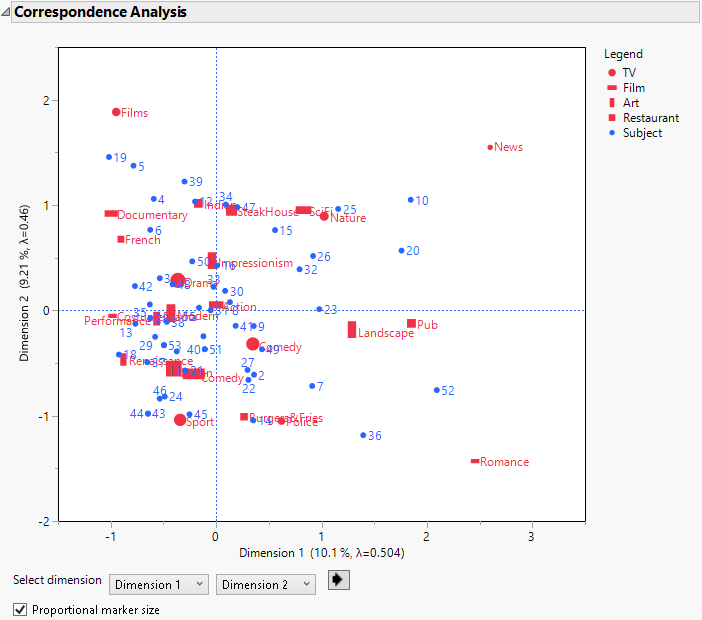
Figure 7.3 Multiple Correspondence Analysis Report with Subjects
Including the subjects highlights a cluster of employees with similar taste in the lower left quadrant of the plot. These employees fall in the area we identified as popular culture.

