Example of Detection Limits
This example illustrates how different detection limits affect process capability results in the Distribution report. The data table in this example contains an actual measurement column as well as four columns with varying levels of a lower limit of detection.
Note: In a real-world situation, you generally have only one measurement column with a specific detection limit. This example uses a hypothetical situation with multiple measurement columns with varying levels of a lower limit of detection for illustration purposes.
1. Select Help > Sample Data Folder and open Impurity Process Capability with Detection Limits.jmp.
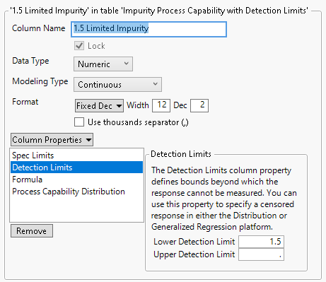
This data table contains four columns with varying levels of a lower limit of detection. For example, in the 1.5 Limited Impurity column, all values of Actual Impurity that are less than 1.5 have been changed to 1.5 and the column has a Detection Limits column property that specifies 1.5 as the Lower Detection Limit, the value below which the response cannot be measured.
2. (Optional.) View the Detection Limits column property for the 1.5 Limited Impurity column.
1. Click on the asterisk icon next to 1.5 Limited Impurity in the Columns panel of the data table window.
2. Select Detection Limits.
Figure 3.24 Column Information Window for 1.5 Limited Impurity Column
3. Click OK.
3. Select Analyze > Distribution.
4. Select Actual Impurity and click Y, Columns.
5. Deselect the Create Process Capability option.
Note: The default process capability analysis is not available for columns that have a Detection Limits column property. For these columns, fit a continuous distribution and then select Process Capability from the red triangle menu within the fitted distribution report. This example uses the Column Switcher to enter columns with a detection limit.
6. Select the Histograms Only option.
7. Click OK.
8. Click the Actual Impurity red triangle and select Continuous Fit > Fit Lognormal.
9. Click the Fitted Lognormal Distribution red triangle and select Process Capability.
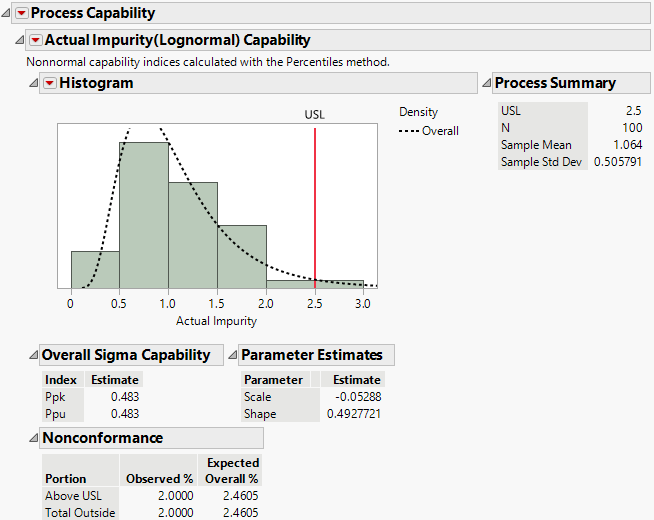
The Process Capability Analysis window uses 2.5 as the upper specification limit. This value comes from the Spec Limits column property for the Actual Impurity column.
10. Click OK.
11. (Optional.) Click the Actual Impurity red triangle and select Histogram Options > Histogram.
Hiding the histogram report frees up space for the process capability analysis.
Figure 3.25 Process Capability Report for Actual Impurity
12. Click the Distributions red triangle and select Redo > Column Switcher.
The Column Switcher enables you to see how different detection limits affect the capability analysis.
13. Select all five columns and click OK.
14. In the Column Switcher, select 1.5 Limited Impurity.
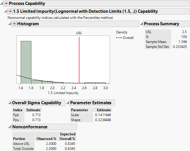
Figure 3.26 Process Capability Report for Impurity with Detection Limit of 1.5
The Process Capability analysis uses a censored lognormal distribution to take into account that the values of 1.5 are censored observations. The report title below Process Capability indicates the detection limits that are present for this analysis.
15. (Optional.) Select other columns in the Column Switcher to investigate how the process capability report changes based on various values of the lower detection limit.
This example enables you to explore how the process capability analysis is affected by increasing amounts of censoring based on a lower detection limit. In general, you would have only one column of observations and one detection limit.


