Summary of Fit Measures
This section describes the summary of fit measures reported in the Structural Equation Models platform.
AICc, BIC, and BICu
The AICc and BIC are defined as follows:
AICc = 
BIC = 
where:
-2logL is twice the negative log-likelihood.
n is the sample size.
k is the number of parameters.
For more information about the likelihood-based measures in the Model Comparisons report, see Likelihood, AICc, and BIC in Fitting Linear Models.
The BIC relative to the unrestricted model (BICu) is defined as follows:
BICu = 
where:
 is the chi-square statistic of the fitted model.
dfmin is the degrees of freedom of the fitted model.
n is the sample size.
The BICu for a fitted model is equivalent to the BIC for the fitted model minus the BIC for the unrestricted model. For more information about the BIC relative to the unrestricted model, see Bollen et al. (2014).
CFI
The comparative fit index (CFI) is defined as follows:
CFI = 
where:
 is the chi-square statistic of the independence model.
df0 is the degrees of freedom of the independence model.
 is the chi-square statistic of the fitted model.
dfmin is the degrees of freedom of the fitted model.
For more information about the CFI, see Bentler (1990).
RNI
The relative noncentrality index (RNI) is defined as follows:
RNI = 
where:
 is the chi-square statistic of the independence model.
df0 is the degrees of freedom of the independence model.
 is the chi-square statistic of the fitted model.
dfmin is the degrees of freedom of the fitted model.
For more information about the RNI, see McDonald and Marsh (1990).
TLI
The Tucker-Lewis index (TLI) is defined as follows:
TLI = 
where:
 is the chi-square statistic of the independence model.
df0 is the degrees of freedom of the independence model.
 is the chi-square statistic of the fitted model.
dfmin is the degrees of freedom of the fitted model.
For more information, see West et al. (2012).
NFI
The Bentler-Bonett normed fit index (NFI) is defined as follows:
NFI = 
where:
 is the chi-square statistic of the independence model.
 is the chi-square statistic of the fitted model.
For more information, see West et al. (2012).
Revised GFI and Revised AGFI
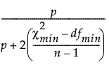
The revised goodness-of-fit index (Revised GFI) is defined as follows:
Revised GFI = 
where:
 is the chi-square statistic of the fitted model.
dfmin is the degrees of freedom of the fitted model.
p is number of observed variables in the fitted model.
n is the sample size.
The revised adjusted goodness-of-fit index (Revised AGFI) is defined as follows:
Revised AGFI = 
where:
p* is the number of unique entries in the covariance matrix and the mean vector of the observed variables.
dfmin is the degrees of freedom of the fitted model.
For more information, see Maiti and Mukherjee (1991) and West et al. (2012).
RMSEA
The root mean square error of approximation (RMSEA) is defined as follows:
RMSEA = 
where:
n is the sample size.
dfmin is the degrees of freedom of the fitted model.
 is the chi-square statistic of the fitted model.
The confidence limits for RMSEA are computed using the cumulative distribution function of the noncentral chi-square distribution Φ(x|λ, d). The 90% confidence limits are computed as follows:
Lower limit = 
Upper limit = 
where:
λL satisfies Φ( |λL, dfmin) = 0.95.
λU satisfies Φ( |λU, dfmin) = 0.05.
For more information, see Maydeu-Olivares et al. (2017).
RMR and SRMR
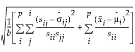
The formulas for RMR and SRMR are defined as follows:
RMR = 
SRMR = 
where:
p is the number of manifest variables.
b is the number of unique entries in the covariance matrix and the mean vector of the observed variables:

sij is the (i, j)th element of the input covariance matrix.
 is the (i, j)th element of the predicted covariance matrix.
 is the ith element of the vector of sample means.
 is the ith element of the vector predicted means.
For more information, see the CALIS Procedure chapter in SAS Institute Inc. (2022a).