Example of a Three-Way Full Factorial Model
Use the Standard Least Squares personality of the Fit Model platform to fit a three-way full factorial model. You are interested in whether speed, angle, and material, or their interactions, have an effect on the amount of wear on a cutting tool.
1. Select Help > Sample Data Folder and open Tool Wear.jmp.
2. Select Analyze > Fit Model.
3. Select Wear and click Y.
4. Select Speed, Angle, and Material and click Macros > Full Factorial.
Note: Effect Screening is automatically selected as the default setting for the Emphasis option in this report. To change to a different report emphasis, you can select either Effect Leverage or Minimal Report for the Emphasis option.
5. Click Run.
6. Click the Response Wear red triangle and select Factor Profiling > Surface Profiler.
Report sections are shown and described below.
Actual by Predicted and Residual Plots
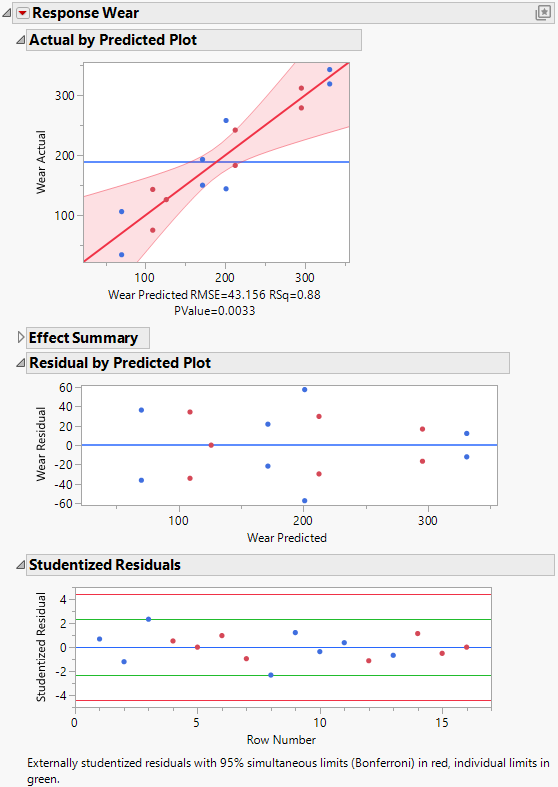
Use the Actual by Predicted and Residual Plots to assess the performance and accuracy of the model.
Figure 4.17 Model Assessment and Diagnostic Plots
The Actual by Predicted Plot indicates that the relationship between the actual and predicted values is statistically significant (p-value = 0.003).
Observe that the Residual by Predicted Plot shows that the residual are randomly scattered and evenly distributed above and below the zero line. This suggests that the model assumptions are met and the residuals are normally distributed.
The Studentized Residuals plot is a scaled version of the residual plot. The residuals fall within the range of –2 to 2, which indicates that the model fits well and the data points are close to the expected values.
Prediction Profiler
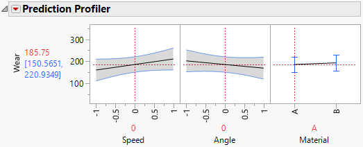
Use the Prediction Profiler to explore how the predicted value of the response varies based on the factor settings.
Figure 4.18 Prediction Profiler
The predicted value of Wear is 185.75 with a 95% confidence interval of 150.57 to 220.93 for a speed of 0, an angle of 0 and Material A.
Tip: To add points to the profiler, select Data Points from the Prediction Profiler red triangle menu.
Surface Profiler
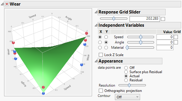
Use the Surface Profiler to explore how the predicted value as a surface of the response varies based on the factor settings.
Figure 4.19 The Surface Profiler
The Surface Profiler shows the predicted response for Wear in terms of the two continuous effects Speed and Angle. Use the slider marked Material in the Independent Variables panel to change the prediction surface from Material A (setting of 0) to Material B (setting of 1). The data points for which Material is A are colored red, whereas those for which Material is B are colored blue. The shape of the surface across the levels of Material is a consequence of the three-way interaction.
Note: The Tool Wear.jmp data table contains data table scripts that generate Surface Profiler plots: Prediction and Surface Profilers and Surface Profilers for Two Materials.


