Additional Example of the Principal Components Platform
Sparse component analysis (SCA) extends principal component analysis (PCA) by focusing on a smaller, more meaningful subset of variables in high-dimensional data. Unlike PCA, which incorporates all variables, SCA selects a subset of variables that contribute most to the principal components, which can improve interpretability. The SCA approach is particularly valuable in fields such as genomics, proteomics, and finance, where data sets often contain a large number of variables but relatively few observations. By identifying the most relevant features, SCA reduces redundancy, highlights key patterns, and ensures that each principal component provides distinct insights. This streamlined approach simplifies analysis, enhances computational efficiency, and makes complex data sets more accessible and interpretable.
In this example, SCA is applied to a proteomics data set that contains 667 protein expression levels from 165 serum samples, including 84 from individuals with prostate cancer and 81 from controls. The objective is to identify key proteins that distinguish between the two groups while reducing the dimensionality of the data. By focusing on proteins that contribute most to the variance, SCA simplifies the data set, which makes it more suitable for downstream tasks such as classification and clustering.
1. Select Help > Sample Data Folder and open Prostate Cancer.jmp.
2. Select Analyze > Multivariate Methods > Principal Components.
3. Select the Proteins column group from the Select Columns list and click Y, Columns.
4. Select Advanced as the Method Family option.
Note: By default, the number of components to be estimated is set to 10. You can modify this value in the text box next to Number of Components based on the context of data and your background knowledge of the study.
Note: The Missing value imputation option is selected by default. It performs data imputation at each iteration of the Sparse Component Analysis algorithm. You can deselect this option if you are confident that there are no missing values in the data set.
5. Select Sparse Components Analysis as the Special Methods option.
6. Click OK.
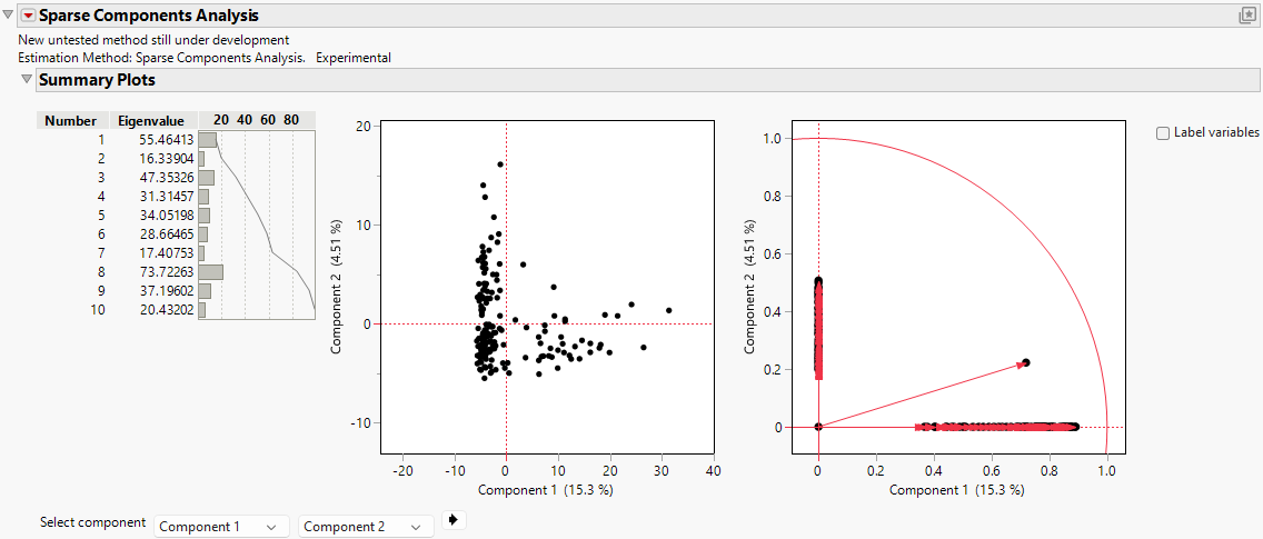
Figure 4.12 Sparse Components Analysis Report
The report includes the eigenvalues and a bar chart of the percentage of variation accounted for by each principal component. Larger eigenvalues indicate greater contributions to the total variance. In this example, Component 8 has the largest eigenvalue (73.72), which indicates that it captures the largest proportion of variance in the data and serves as the most informative component to explain the underlying data structure. Components 1 (55.46), 3 (47.35), 9 (37.20), and 5 (34.05) also have relatively high eigenvalues, which indicates that they are significant contributors to the variability of the data set. Together, these components account for a substantial portion of the variance.
Components 4 (31.31) and 6 (28.66) have moderate eigenvalues, which suggests that they contribute meaningful but less dominant variance. However, Components 2 (16.34), 7 (17.41), and 10 (20.43) show the lowest eigenvalues, which reflect limited contributions to the total variance. These components with smaller eigenvalues might capture finer or less significant aspects of the data.
The concentration of variance in a few components, particularly Component 8, highlights the effectiveness of SCA in finding key patterns while reducing dimensionality. The sparsity that is enforced by SCA ensures that the identified components focus on the most significant features, which makes them interpretable and computationally efficient. You might prioritize components with larger eigenvalues for further investigation, because they encapsulate the most critical variations associated with prostate cancer characteristics.
7. Click the Sparse Components Analysis red triangle and select Loading Matrix.
8. Click the gray disclosure icon next to Loading Matrix.
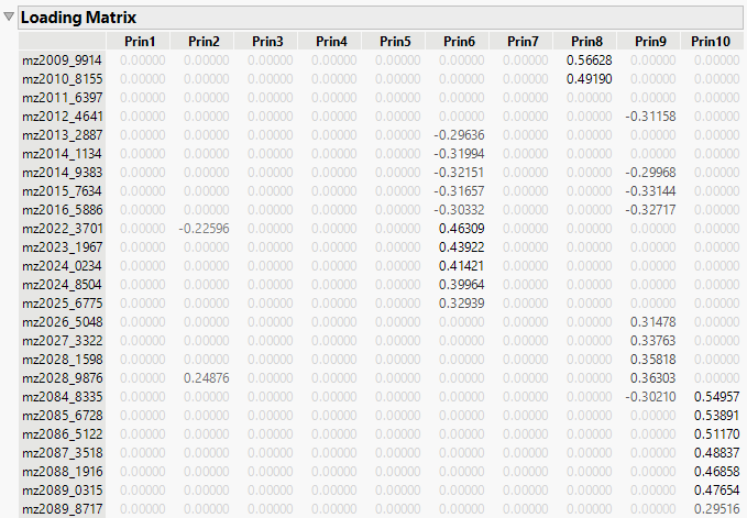
Figure 4.13 Sparse Components Analysis Loading Matrix (partial)
The loading matrix represents the contributions of the original variables to the derived principal components. The loading matrix enables you to identify dimensions where specific variables have either a dominant or negligible influence. For example, in Component 8 (Prin8), the variable mz4062_2282 has a loading of approximately 1.05870, which is significantly higher than the contributions of other variables. This suggests that mz4062_2282 is a dominant variable in explaining the variance that is captured by Component 8. Similarly, in Prin10, the variable mz2084_8335 has a loading of 0.54957, which indicates that it has substantial influence on this component.
Moreover, variables with loadings that are close to zero contribute minimally to the variance explained by a principal component. For example, variables such as mz2011_6397 have zero loadings across all principal components, which suggests that they do not significantly contribute to the variance that is captured by the model. These insights can inform decisions about variable importance or potential redundancy.

