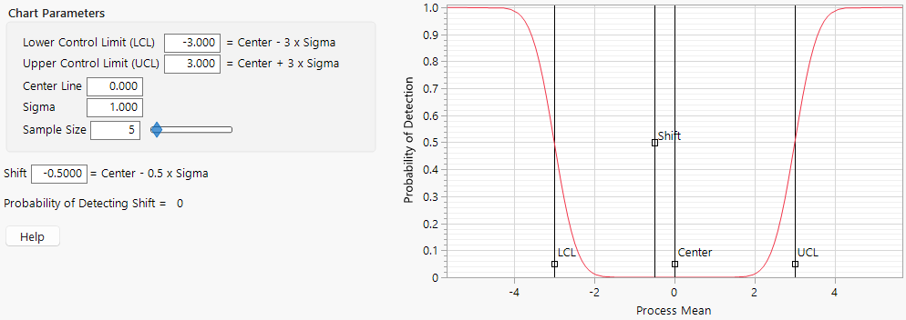
Example of Operating Characteristic Curves

Use the OC Curve platform to estimate the probability of identifying a process shift with the first sample collected after the shift.

1. Select Analyze > Quality and Process > OC Curves.

2. Select XBar Shewhart Chart.

3. Click OK.

Figure 17.1 OC Curve Default Setting 

The vertical axis is the probability of detecting a shift. Note that the probability of detecting a shift of -0.5 for limits of 3 is 0. A shift of -0.5 is unlikely to be detected with a sample size of 5.

4. Set the control limits to -1.34 and 1.34. These are 3 sigma limits for s = 1 and n = 5 (3 times 1 divided by the square root of 5).

5. Leave Sigma set to 1 and the sample size at 5.

6. Set Shift to 2.

Notice that the probability of detection is now 0.93. The probability of detecting a shift of size 2s with a sample of size 5 is 1 - 0.07 = 0.93.