Parametric Tolerance Intervals
Use the Parametric Tolerance Intervals Explorer to determine a sample size for tolerance intervals. A tolerance interval contains a portion of the population p with 100(1 – α) confidence. Select DOE > Sample Size Explorers > Reliability > Parametric Tolerance Intervals. Explore the trade-offs between sample size, significance, variability assumption, and the interval margin.
Parametric Tolerance Intervals Explorer
Set study assumptions and explore sample sizes by using the radio buttons, text boxes, and menus. The profiler updates as you make changes to the settings. Alternatively, you can change the settings by dragging the cross hairs on the profiler curves.
Interval Type
Specifies the type of interval. Specify Upper Bound or Lower Bound for a one-sided interval. Specify Interval for a two-sided interval.
Confidence Level
Specifies the confidence level, 1 – α.
Distribution
Specifies the distribution for the population. Distribution options include Normal, Lognormal, Exponential, Weibull, and SEV.
Proportion
Specifies the proportion of the population for the interval to cover.
Parametric Tolerance Intervals Explorer Profiler
The profiler enables you to visualize the impact of sample size assumptions on the interval margin calculations. Interactive profiler changes to the sample size or sigma update the calculated interval margin. Interactive changes to the profiler interval margin update the sample sizes. To solve for a specific variable, use the target variable setting and click Go.
Target Variable
Enables you to solve for the sample size.
Interval Margin
Specifies the difference between the width of the tolerance interval constructed from a sample of size N and the width of the theoretical tolerance interval. With all other parameters fixed, the interval margin decreases as sample size increases.
Sample Size
Specifies the total number of observations (runs, experimental units, or samples) that are needed to construct your interval.
Sigma
(Not available for Exponential and Weibull distributions.) Specifies the assumed population standard deviation.
Scale Parameter
(Available only for Exponential and Weibull distributions.) Specifies the scale parameter for the distribution.
Beta
(Available only for the Weibull distributions.) Specifies Beta, the rate parameter for the Weibull distribution.
Parametric Tolerance Intervals Explorer Options
The Explorer red triangle menu and report buttons provide additional options:
Simulate Data
Opens a data table of simulated data that are based on the explorer settings. View the simulated response column formula for the settings that are used. Run the table script to analyze the simulated data.
Make Data Collection Table
Creates a new data table that you can use for data collection. The table includes scripts to facilitate data analysis.
Remember Settings
Saves the current settings to the Remembered Settings table. This enables you to save a set of alternative study plans. See Remembered Settings in the Sample Size Explorers.
Reset to Defaults
Resets all parameters and graphs to their default settings.
The Profiler red triangle menu contains the following option:
Optimization and Desirability
Enables you to optimize settings. See “Desirability Profiling and Optimization” in Profilers.
Note: The sample size explorer report can be saved as a *.jmpdoe file. Open the file to return to the explorer. An alert prompts you to save the file.
Example of the Parametric Tolerance Intervals Explorer
In this example, use the Parametric Tolerance Intervals Explorer to explore the interval margin for a tolerance interval to cover 90% of your population with 95% confidence.
Recall that the interval margin is the difference between the width of the theoretical tolerance interval and the width of the estimated tolerance interval. For a normal distribution with mean = 0 and standard deviation (sigma) = 1, the theoretical tolerance interval to cover 90% of the population is -1.645 to 1.645. Therefore, the width is 3.29.
1. Select DOE > Sample Size Explorers > Reliability > Parametric Tolerance Intervals.
2. Leave Interval Type set to Interval for estimating a sample size for a two-sided tolerance interval.
3. Leave Confidence Level set to 0.95.
4. Leave Distribution set to Normal.
5. Leave Proportion set to 0.9.
6. Leave Target Variable set to Sample Size.
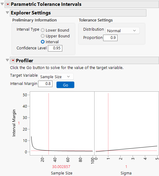
7. Set Interval Margin to 1.
8. In the profiler, leave Sigma set to 1.
9. Click Go.
Figure 29.11 Parametric Tolerance Intervals Explorer
A sample size of 30 allows the estimation of a tolerance interval to cover 90% of the population with 95% confidence. This tolerance interval has a width within 1 unit of the theoretical tolerance interval.
10. Select Simulate Data from the Parametric Tolerance Intervals red triangle.
11. Run the Distribution table script.
Figure 29.12 Parametric Tolerance Interval Simulation
With a sample size of 30, a simulated tolerance interval has a width of 1.88 - (-2.48) = 4.36. This width is approximately 1 unit greater than the theoretical tolerance interval width of 3.29.
Note: Your results can differ due to the randomness of the simulation.
Statistical Details for the Parametric Tolerance Intervals Explorer
The Interval Margin is the difference between the expected width of the tolerance interval given the sample size and the corresponding theoretical tolerance interval.
Assuming a normal distribution, a two-sided tolerance interval to cover proportion q of the population the tolerance interval is calculated as follows:

For a one-sided tolerance interval to cover proportion q of the population the tolerance intervals is calculated as follows:

where:
μ is the mean of the sample
α is the significance level
zα is the αth quantile of the normal distribution
χ2α,ν is the αth quantile of a central χ2 distribution with ν degrees of freedom
t1-α,ν is the (1 - α)th quantile of the central t-distribution with ν degrees of freedom
σ is the assumed population standard deviation
n is the number of samples.
For a lognormal distribution, use the same formulas as above, taking the exponential before computing the margin.
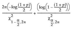
For the exponential distribution, the lower bound factor is given by

and the upper bound factor is given by

and the relative interval width is given by

Each of these quantities are multiplied by the scale factor. For more information about exponential bounds see Blischke and Murthy (2000).
For the SEV distribution, the tolerance factors are approximated by upper tolerance factor:

and the lower tolerance factor:

where


and

For more information see Bain and Englehardt (1981).

