Power for Two Independent Sample Means
Use the Power for Two Independent Sample Means Explorer to determine a sample size for a hypothesis test about the means from two groups. Select DOE > Sample Size Explorers > Power > Power for Two Independent Sample Means. Explore the trade-offs between sample size, power, significance, and the hypothesized difference to detect. Sample size and power are associated with the following hypothesis test:

versus the two-sided alternative:

or versus a one-sided alternative:
 or
or 
where μ1 and μ2 are the true means of the two populations. It is assumed that the populations of interest are normally distributed and that you want to detect a difference of δ between the means.
Power Explorer for Two Independent Sample Means Settings
Set study assumptions and explore sample sizes by using the radio buttons, text boxes, and menus. The profiler updates as you make changes to the settings. Alternatively, you can change the settings by dragging the cross hairs on the profiler curves.
Test Type
Specifies a one- or two-sided hypothesis test.
Alpha
The probability of a type I error, which is the probability of rejecting the null hypothesis when it is true. It is commonly referred to as the significance level of the test. The default alpha level is 0.05.
Population Standard Deviation Assumption
Specifies the distribution for calculations.
No
Specifies an unknown standard deviation; calculations use the t distribution. This is common.
Yes
Specifies a known standard deviation; calculations use the z distribution.
Power Explorer for Two Independent Sample Means Profiler
The profiler enables you to visualize the impact of sample size assumptions on the power calculations. Interactive profiler changes to the sample sizes, difference to detect, or standard deviations update the calculated power. Interactive changes to the profiler power update the sample sizes. To solve for a specific variable, use the target variable setting and click Go.
Target Variable
Enables you to solve for a sample size, difference to detect, or an assumed group standard deviation at a specified power.
Power
Specifies the probability of rejecting the null hypothesis when it is false. With all other parameters fixed, power increases as sample size increases.
Ratio of Group 2 to Group 1 Sample Size
Specifies the ratio between group sample sizes. For equal group sample sizes, set this option to 1.
Note: The ratio can shift as you explore changes to the assumptions due to the mathematical search routines.
Total Sample Size
Specifies the total number of observations (runs, experimental units, or samples) that are needed for your experiment.
Group 1 Sample Size
Specifies the number of observations (runs, experimental units, or samples) that are needed for Group 1 in your experiment.
Group 2 Sample Size
Specifies the number of observations (runs, experimental units, or samples) that are needed for Group 2 in your experiment.
Difference to Detect
Specifies the smallest difference between the group means that you want to be able to declare statistically significant.
Group 1 StdDev (Noise)
Specifies the assumed standard deviation for one of your groups, Group 1. An estimate of the error standard deviation could be the root mean square error (RMSE) from a previous model fit.
Group 2 StdDev (Noise)
Specifies the assumed standard deviation for the second group, Group 2. An estimate of the error standard deviation could be the root mean square error (RMSE) from a previous model fit.
Power Explorer for Two Independent Sample Means Options
The Explorer red triangle menu and report buttons provide additional options:
Simulate Data
Opens a data table of simulated data that are based on the explorer settings. View the simulated response column formula for the settings that are used. Run the table script to analyze the simulated data.
Make Data Collection Table
Creates a new data table that you can use for data collection. The table includes scripts to facilitate data analysis.
Remember Settings
Saves the current settings to the Remembered Settings table. This enables you to save a set of alternative study plans. See Remembered Settings in the Sample Size Explorers.
Reset to Defaults
Resets all parameters and graphs to their default settings.
The Profiler red triangle menu contains the following option:
Optimization and Desirability
Enables you to optimize settings. See “Desirability Profiling and Optimization” in Profilers.
Note: The sample size explorer report can be saved as a *.jmpdoe file. Open the file to return to the explorer. An alert prompts you to save the file.
Example of Power Explorer for Two Independent Sample Means
In this example, use the Power Explorer for Two Independent Sample Means to determine the number of units to test in a study of two treatments. Suppose that you are interested in demonstrating that the means of two treatment groups are at least 2 standard deviation units apart. You would like to design an experiment that has 85% power to detect a difference of 2 standard deviation units between the means of the two groups at a significance level of α = 0.05.
1. Select DOE > Sample Size Explorers > Power > Power for Two Independent Sample Means.
2. Leave Test Type set to Two-Sided.
3. Leave Alpha set to 0.05.
4. Leave the population standard deviation assumption set to No. Sample size is calculated using the t distribution.
5. Leave Target Variable set to Total Sample Size.
6. Enter 0.85 for Power.
7. In the profiler, leave the Group 1 Std Dev (Noise) and Group 2 Std Dev (Noise) values set to 1.
8. In the profiler, use the slider or click on the red value for a text box to set the Difference to Detect to 2.
9. Click Go.
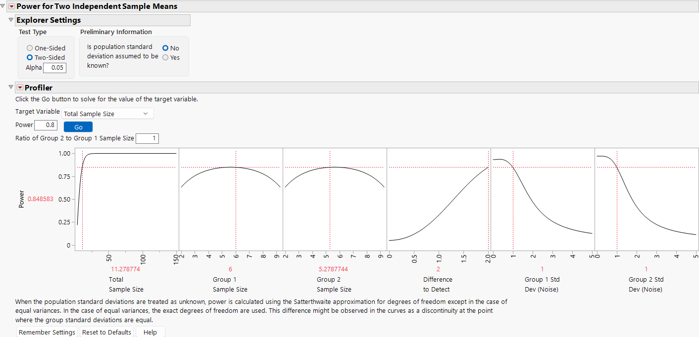
Figure 29.4 Two Independent Sample Means Explorer
Note that a sample size is not a whole number. In practice, round the total sample size up to 12 with 6 per group. This results in a power of 0.876, which is above your minimum required power of 0.85.
10. (Optional) Click Remember Settings to save these settings with a setting name that you can specify.
11. (Optional) Use the profiler to explore other sample size and power possibilities for your study.
12. (Optional) If desired, save the power explorer to a *.jmpdoe file to revisit the settings later.
13. (Optional) Select Make Data Collection Table from the Power for Two Independent Means red triangle to create a data table for data collection. After data collection, use the table script to run your analysis.
Statistical Details for the Power Explorer for Two Independent Sample Means
The power calculations for testing the difference in means of two sample groups are based on the traditional t test, or if σ1 and σ2 are known, the z test.
Variances Unknown
For the case when the group variances are unknown, it is assumed that σ1=σ2=σ and the power is calculated based on the form of the alternative hypothesis.
For a one-sided, higher alternative (μ1 > μ2):

For a one-sided, lower alternative (μ1 < μ2):

For a two-sided alternative (μ1 ≠ μ2):


where:
α is the significance level
n1 and n2 are the group sample sizes
σ is the pooled standard deviation
δ is the difference to detect
t1-α,ν is the (1 - α)th quantile of the central t-distribution with ν degrees of freedom
T(t; ν, λ) is the cumulative distribution function of the non-central t distribution with ν degrees of freedom and non-centrality parameter λ.
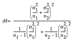
The degrees of freedom are approximate degrees of freedom, also known as Satterthwaite degrees of freedom:

The power calculations are conservative when the variances are equal. However, assuming unequal variances provides a more robust sample size estimate than assuming equal variances.
Variances Known
When σ1 and σ2 are known the z distribution is used for the power calculation. The power is calculated based on the form of the alternative hypothesis.
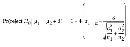
For a one-sided, higher alternative (μ1 > μ2):

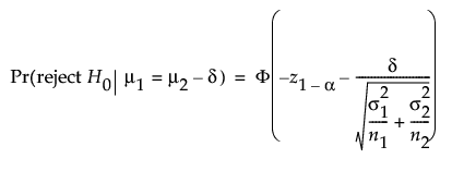
For a one-sided, lower alternative (μ1 < μ2):

For a two-sided alternative (μ1 ≠ μ2):

where:
α is the significance level
n1 and n2 are the group sample sizes
σ1 and σ2 are known group standard deviations
δ is the difference to detect
z1-α is the (1 - α)th quantile of the z-distribution
Φ(x) is the cumulative distribution function of the normal distribution.
