Statistical Details for Continuous Distributions
This section contains statistical details for the options in the Continuous Fit menu in the Distribution platform. Unless otherwise specified, confidence intervals for parameter estimates use likelihood-based calculations. For more information about likelihood-based confidence intervals, see “Statistical Details for Profile Likelihood Confidence Limits” in Predictive and Specialized Modeling. If the Y column has a Detection Limits column property, the Continuous Fit options fit a censored distribution and only a subset of distributions are available. For more information about fitting distributions to censored data, see Meeker and Escobar (1998).
Normal
The normal distribution is defined by two parameters:
• μ (the mean) defines the location of the distribution on the x-axis
• σ (standard deviation) defines the dispersion or spread of the distribution
The standard normal distribution occurs when μ = 0 and σ = 1.
pdf:  for
for  ;
;  ; 0 < σ
E(x) = μ
Var(x) = σ2
Note: Confidence intervals for the mean estimate are based on the t distribution. Confidence intervals for the scale parameter are based on the χ2 distribution.
Cauchy
The Cauchy distribution is a unimodal, symmetric distribution with heavier tails than the normal distribution. The Cauchy distribution is defined by two parameters; location μ and scale σ.
pdf:  for
for  ;
;  ; 0 < σ
E(x) = undefined
Var(x) = undefined
Student’s t
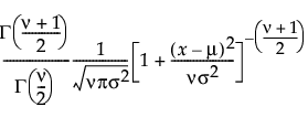
The Student’s t distribution is defined by three parameters; location μ, scale σ, and degrees of freedom ν.
pdf:  for
for  ;
;  ; 0 < σ; 1 ≤ ν
E(x) = μ for 1 < ν
Var(x) = σ2ν/(ν-2) for 2 < ν
Note: When ν = 1, the Student’s t distribution is equivalent to the Cauchy distribution.
SHASH
The sinh-arcsinh (SHASH) distribution is based on a transformation of the normal distribution and includes the normal distribution as a special case. It can be symmetric or asymmetric. The SHASH distribution is defined by four parameters; location θ, scale σ, and two shape parameters, γ and δ. For more information about the SHASH distribution, see Jones and Pewsey (2009).
pdf:  for
for  ; 0 < δ, σ
where
 is the standard normal pdf

• When γ = 0 and δ = 1, the SHASH distribution is equivalent to the normal distribution with location θ and scale σ.
• The transformation sinh(w) is normally distributed with μ = 0 and σ = 1.
ZI SHASH
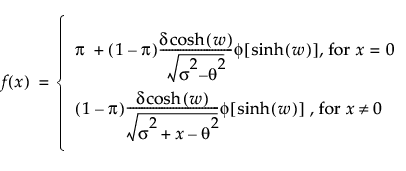
The zero-inflated (ZI) sinh-arcsinh (SHASH) distribution is a SHASH distribution with a point mass at zero. It can be symmetric or asymmetric. The ZI SHASH distribution is defined by five parameters; location θ, scale σ, two shape parameters, γ and δ, and the zero-inflation proportion π.
pdf:  for
for  ; 0 < δ, σ
where
 is the standard normal pdf

Note: Confidence intervals for ZI SHASH distribution parameter estimates use Wald-based calculations.
Exponential
The exponential distribution is especially useful for describing events that randomly occur over time, such as survival data. The exponential distribution might also be useful for modeling elapsed time between the occurrence of non-overlapping events. Examples of non-overlapping events include the following: the time between a user’s computer query and response of the server, the arrival of customers at a service desk, or calls coming in at a switchboard.
The exponential distribution is a special case of the two-parameter Weibull when β = 1 and α = σ, and also a special case of the Gamma distribution when α = 1.
pdf:  for 0 < σ; 0 ≤ x
E(x) = σ
Var(x) = σ2
Devore (1995) notes that an exponential distribution is memoryless. Memoryless means that if you check a component after t hours and it is still working, the distribution of additional lifetime (the conditional probability of additional life given that the component has lived until t) is the same as the original distribution.
ExGaussian
The ExGaussian distribution is the sum of a normal distribution and an exponential distribution. The ExGaussian distribution is defined by the location μ, and scale σ, parameters of the normal distribution and the exponential distribution parameter λ.
pdf:  for
for  ;
;  ; 0 < σ, λ
where Φ(·) is the standard normal cdf.
E(x) = μ + 1/λ
Var(x) = σ2 + 1/λ2
For more information about the exponentially modified Gaussian distribution, see Ament et al. (2019) and Palmer et al. (2011). Note that the parameterization of the exponential portion of the distribution differs in some sources. The parameterization in the Fit ExGaussian option uses the reciprocal of the parameterization that is used in the Fit Exponential option in the Distribution platform.
Gamma
The gamma distribution is defined by two parameters; shape α and scale σ, both positive. The distribution is restricted to positive data.
pdf:  for 0 < x; 0 < α, σ
E(x) = ασ
Var(x) = ασ2
• The standard gamma distribution has σ = 1. Values other than 1 stretch or compress the distribution along the horizontal axis.
• The chi-square  distribution is a special case of the gamma distribution when σ = 2 and α = ν/2.
• The exponential distribution is a special case of the gamma distribution when α = 1.
The standard gamma density function is strictly decreasing when α ≤ 1. When α > 1, the density function begins at zero, increases to a maximum, and then decreases.
Lognormal
The Lognormal distribution is defined by two parameters; scale μ and shape σ. A variable Y is lognormal if and only if X = ln(Y) is normal. The distribution is restricted to positive data.
pdf:  for
for  ;
;  ; 0 < σ
E(x) = 
Var(x) = 
Weibull
The Weibull distribution is defined by two parameters; scale α and shape β. It often provides a good model for estimating the length of life, especially for mechanical devices and in biology.
The pdf for the Weibull distribution is defined as follows:
pdf:  for α,β > 0; 0 < x
E(x) = 
Var(x) = 
where Γ(·) is the Gamma function.
Smallest Extreme Value
The Smallest Extreme Value (SEV) distribution is defined by two parameters; location μ, and scale σ. The SEV distribution is a non-symmetric, left-skewed distribution and is useful when the standard deviation is small relative to the mean. This distribution is also known as the Gumbel distribution.
pdf:  for
for  ; 0 < σ
E(x) = 
Var(x) = 
where

and γ is Euler’s constant.
Largest Extreme Value
The Largest Extreme Value (LEV) distribution is defined by two parameters; location μ, and scale σ. The LEV distribution is a non-symmetric, right-skewed distribution and is often used to model natural extreme phenomena, such as catastrophic flood heights or extreme wind velocities. This distribution is also known as the Gumbel distribution.
pdf:  for
for  ; 0 < σ
E(x) = 
Var(x) = 
where

and γ is Euler’s constant.
Normal 2 Mixture and Normal 3 Mixture
The Normal 2 Mixture and Normal 3 Mixture distributions are defined by two or three location μi, scale σi, and proportion πi parameter sets. These flexible distributions are capable of fitting bimodal or multi-modal data.
pdf: 
E(x) =
Var(x) =
where μi, σi, and πi are the respective mean, standard deviation, and proportion for the ith group, φ(·) is the standard normal pdf, and k is the number of normal distributions in the mixture.
Note: Confidence intervals for normal mixture distribution parameter estimates use Wald-based calculations.
Johnson
The Johnson system of distributions contains three distributions that are based on a transformed normal distribution. These three distributions are the following:
• Johnson Su, which is unbounded and defined by four parameters; location θ, scale σ, and two shape parameters, γ and δ.
• Johnson Sb, which has bounds on both tails and defined by four parameters; location θ, scale σ, and two shape parameters, γ and δ.
• Johnson Sl, which is bounded in one tail and defined by three parameters; scale σ, and two shape parameters, γ and δ. The Johnson Sl family contains the family of lognormal distributions.
Only the fit for the best fitting Johnson distribution is reported. Information about selection procedures and parameter estimation for the Johnson distributions can be found in Slifker and Shapiro (1980). The parameter estimation does not use maximum likelihood.
Johnson distributions are popular because of their flexibility. In particular, the Johnson distribution system is noted for its data-fitting capabilities because it supports every possible combination of skewness and kurtosis. However, the SHASH distribution is also very flexible and is recommended over the Johnson distributions.
If Z is a standard normal variate, then the system is defined as follows:

where, for the Johnson Su:


where, for the Johnson Sb:


and for the Johnson Sl, where σ = ±1.


Johnson Su
pdf:  for -∞ < x, θ, γ < ∞; 0 < θ,δ
Johnson Sb
pdf:  for θ < x < θ+σ; 0 < σ
Johnson Sl
pdf:  for θ < x if σ = 1; θ > x if σ = -1
where φ(·)is the standard normal pdf.
Note: Confidence intervals for Johnson distribution parameter estimates use Wald-based calculations.
Beta
The Beta distribution is defined by two shape parameters, α > 0 and β > 0. The beta distribution takes on values in the interval 0 to 1.The beta distribution is useful for modeling the behavior of random variables that are constrained to the interval 0 to 1. For example, proportions always fall between 0 and 1.
pdf:  for 0 < x < 1; 0 < σ,α,β
E(x) = 
Var(x) = 
where B(·) is the Beta function.
AICc and BIC
In the Compare Distributions report, the Distribution list includes AICc and BIC criterion.
The formulas for AICc and BIC are defined as follows:
AICc = 
BIC = 
where:
– logL is the log-likelihood.
– n is the sample size.
– k is the number of parameters.
The AICc Weight column shows normalized AICc values that sum to one. The AICc weight can be interpreted as the probability that a particular distribution is the true distribution given that one of the fitted distributions is the truth. Therefore, the distribution with the AICc weight closest to one is the better fit. The AICc weights are calculated using only nonmissing AICc values:
AICcWeight = exp[-0.5(AICc-min(AICc))] / sum(exp[-0.5(AICc-min(AICc))])
where min(AICc) is the smallest AICc value among the fitted distributions.
For more information about the measures in the Compare Distributions report, see “Likelihood, AICc, and BIC” in Fitting Linear Models.