In the early stages of studying a process, you identify a list of factors that potentially affect your response or responses. You are interested in identifying the active factors, that is, the factors that actually do affect your response or responses. A screening design helps you determine which factors are likely to be active. Once the active factors are identified, you can construct more sophisticated designs, such as response surface designs, to model interactions and curvature.
The Custom Design platform constructs screening designs using either the D-optimality or Bayesian D-optimality criterion. The D-optimality criterion minimizes the determinant of the covariance matrix of the model coefficient estimates. It follows that D-optimality focuses on precise estimates of the effects. For details, see Optimality Criteria in Custom Designs.
|
1.
|
Select DOE > Custom Design.
|
|
2.
|
In the Factors outline, type 6 next to Add N Factors.
|
|
3.
|
Click Add Factor > Continuous.
|
|
4.
|
Click Continue.
|
Note: Setting the Random Seed in step 5 and Number of Starts in step 6 reproduces the exact results shown in this example. When constructing a design on your own, these steps are not necessary.
|
5.
|
(Optional) From the Custom Design red triangle menu, select Set Random Seed, type 1839634787, and click OK.
|
|
6.
|
|
7.
|
Click Make Design.
|
|
8.
|
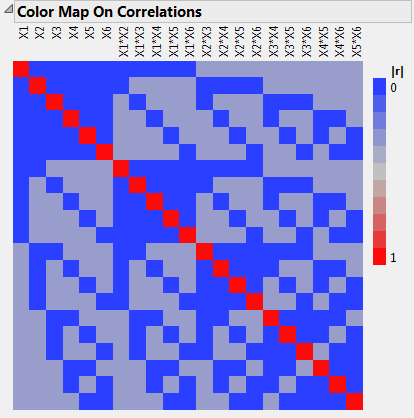
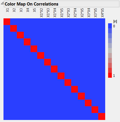
Open the Design Evaluation > Color Map on Correlations outline.
|
|
9.
|
Open the Design Evaluation > Alias Matrix outline.
|
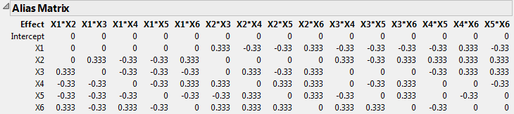
The Alias Matrix shows how the coefficients of the main effect terms in the model are biased by potentially active two-factor interaction effects. The column labels identify interactions. For example, in the X1 row, the column X2*X3 has a value of 0.333 and the column X2*X4 has a value of -0.33. This means that the expected value of the main effect of X1 is the sum of the main effect of X1 plus 0.333 times the effect of X2*X3, plus -0.33 times the effect of X2*X4, and so on, for the rest of the X1 row. In order for the estimate of the main effect of X1 to be meaningful, you must assume that these interactions are negligible in size compared to the effect of X1.
Tip: The Alias Matrix is a generalization of the confounding pattern in fractional factorial designs.
The Alias Matrix in Alias Matrix shows partial aliasing of effects. In other cases, main effects might be fully aliased, or confounded, with two-factor interactions. In both of these cases, strong two-factor interactions can confuse the results of main effects only experiments. To avoid this risk, create a design that resolves all two-factor interactions.
|
1.
|
Select DOE > Custom Design.
|
|
2.
|
Type 5 next to Add N Factors.
|
|
3.
|
Click Add Factor > Continuous.
|
|
4.
|
Click Continue.
|
|
5.
|
In the Model outline, select Interactions > 2nd.
|

|
6.
|
Click Minimum to accept 16 for the number of runs.
|
Note: Setting the Random Seed in step 7 and Number of Starts in step 8 reproduces the exact results shown in this example. In constructing a design on your own, these steps are not necessary.
|
7.
|
(Optional) From the Custom Design red triangle menu, select Set Random Seed, type 819994207, and click OK.
|
|
8.
|
|
9.
|
Click Make Design.
|
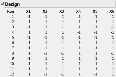
Design to Estimate All Two-Factor Interactions shows the runs of the design. All main effects and two-factor interactions are estimable because their Estimability was designated as Necessary (by default) in the Model outline.

|
10.
|
Open the Design Evaluation > Color Map on Correlations outline.
|
In this example, you find a compromise between an 8-run main effects only design (see Design That Estimates Main Effects Only) and a 22-run design capable of fitting all the two-factor interactions. You use Alias Optimality as the optimality criterion to achieve your goal.
|
1.
|
Select DOE > Custom Design.
|
|
2.
|
Type 6 next to Add N Factors.
|
|
3.
|
Click Add Factor > Continuous.
|
|
4.
|
Click Continue.
|
|
5.
|
Select Optimality Criterion > Make Alias Optimal Design from the red triangle menu.
|
The Make Alias Optimal Design selection tells JMP to generate a design that balances reduction in aliasing with D-efficiency. See Alias Optimality in Custom Designs.
|
6.
|
Click User Specified and change the number of runs to 16.
|
Note: Setting the Random Seed in step 7 and Number of Starts in step 8 reproduces the exact results shown in this example. In constructing a design on your own, these steps are not necessary.
|
7.
|
(Optional) From the Custom Design red triangle menu, select Set Random Seed, type 1692819077, and click OK.
|
|
8.
|
(Optional) From the Custom Design red triangle menu, select Number of Starts, type 161, and click OK.
|
|
9.
|
Click Make Design.
|
|
10.
|
Open the Design Evaluation > Alias Matrix outline.
|
|
11.
|
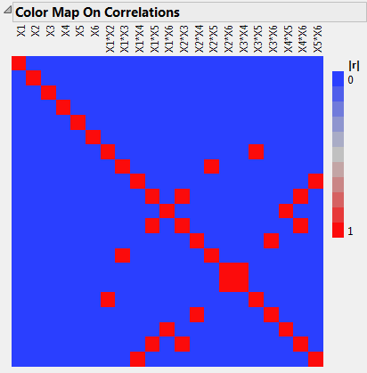
Open the Design Evaluation > Color Map on Correlations outline.
|
In a saturated design, the number of runs equals the number of model terms. In a supersaturated design, the number of model terms exceeds the number of runs (Lin, 1993). A supersaturated design can examine dozens of factors using fewer than half as many runs as factors. This makes it an attractive choice for factor screening when there are many factors and experimental runs are expensive.
|
•
|
If the number of active factors is more than half the number of runs in the experiment, then it is likely that these factors will be impossible to identify. A general rule is that the number of runs should be at least four times larger than the number of active factors. In other words, if you expect that there might be as many as five active factors, you should plan on at least 20 runs.
|
|
•
|
Analysis of supersaturated designs cannot yet be reduced to an automatic procedure. However, using forward stepwise regression is reasonable. In addition, the Screening platform (Analyze > Modeling > Screening) offers a streamlined analysis.
|
Note: This example is for illustration only. You should have at least 14 runs in any supersaturated design. If there are as many as four active factors, it is very difficult to interpret the results of an 8-run design. See Limitations of Supersaturated Designs.
|
1.
|
Select DOE > Custom Design.
|
|
2.
|
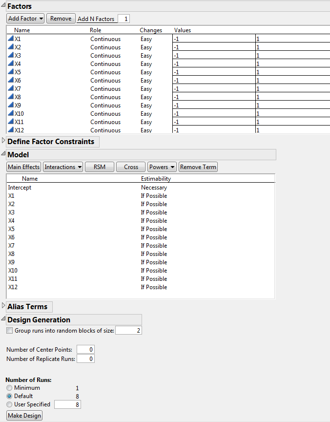
Type 12 next to Add N Factors.
|
|
3.
|
Click Add Factor > Continuous.
|
|
4.
|
Click Continue.
|
|
6.
|
|
7.
|
|
8.
|
Select Simulate Responses from the red triangle menu.
|
Note: Setting the Random Seed in step 9 and Number of Starts in step 10 reproduces the exact results shown in this example. In constructing a design on your own, these steps are not necessary.
|
9.
|
(Optional) From the Custom Design red triangle menu, select Set Random Seed, type 1008705125, and click OK.
|
|
10.
|
(Optional) From the Custom Design red triangle menu, select Number of Starts, type 100, and click OK.
|
|
11.
|
Click Make Design.
|
|
12.
|
Click Make Table.
|
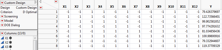
The design table (Design Table with Simulated Responses) and the Simulate Responses window (Simulate Responses Window) appear.

The response column, Y, contains simulated values. These are randomly generated using the model defined by the parameter values in the Simulate Responses window.
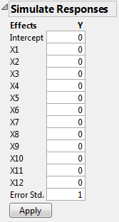
The Simulate Responses window shows coefficients of 0 for all terms, with an Error Std of 1. The values in the Y column currently reflect only random variation. Notice that the model coefficients are set to 0 because not all coefficients are estimable.
|
13.
|
|
14.
|
Click Apply.
|
Note: If you did not set the random seed and the number of starts, or if you click Apply more than once, your response values will not match those in Response Column with X1 and X11 Active.
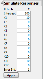
In your simulation, you specified X1 and X11 as active factors with large effects relative to the error variation. For this reason, your analysis of the data should identify these two factors as active.
The Screening platform provides a way to identify active factors. The design table in Response Column with X1 and X11 Active contains three scripts. The Screening script analyzes your data using the Screening platform (located under the Analyze > Modeling > Screening menu).
|
1.
|
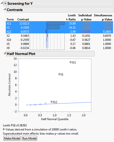
The factors X1 and X11 have large contrast and Lenth t-Ratio values. Also, their Simultaneous p-Values are small. In the Half Normal Plot, both X1 and X11 fall far from the line. The Contrasts and the Half Normal Plot reports indicate that X1 and X11 are active. Although X12 has an Individual p-Value less than 0.05, its effect is much smaller than that of X1 and X11.
Because the design is supersaturated, p-values might be smaller than they would be in a model where all effects are estimable. This is because effect estimates are biased by other potentially active main effects. In Screening Report for Supersaturated Design, a note directly above the Make Model button warns you of this possibility.
You might also want to check whether the effects that appear active could be highly correlated with other effects. When this occurs, one effect can mask the true significance of another effect. See step 4.
|
2.
|
Click Make Model.
|
|
3.
|
Click Run in the Model Specification window.
|
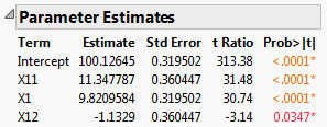
Note that the parameter estimates for X11 and X1 are close to the theoretical values that you used to simulate the model. See Parameter Values for Simulated Responses, where you specified a model with X1 = 10 and X11 = 10. The significance of the factor X12 is an example of a false positive.
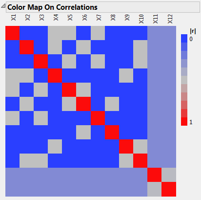
With your cursor, place your mouse pointer over cells to see the absolute correlations. Notice that X1 has correlations as high as 0.5 with other main effects (X4, X5, X7).
Stepwise regression is another way to identify active factors. The design table in Response Column with X1 and X11 Active contains three scripts. The Model script analyzes your data using stepwise regression in the Fit Model platform.
|
1.
|
|
2.
|
|
3.
|
Click Run.
|
|
4.
|
|
5.
|
Click Go.
|
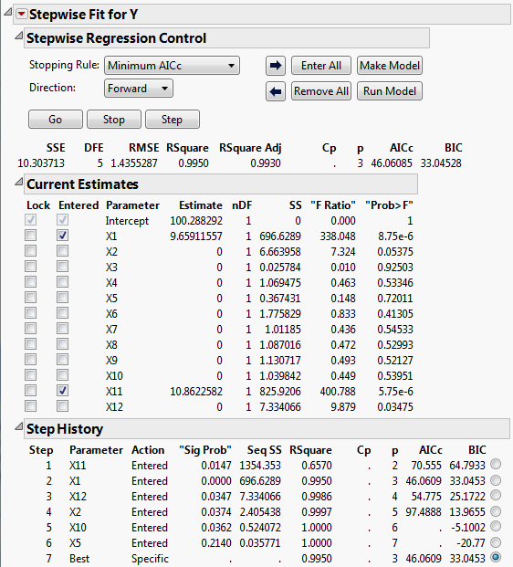
Stepwise Regression for Supersaturated Design shows that the selected model consists of the two active factors, X1 and X11. The step history appears in the bottom part of the report. Keep in mind that correlations between X1 and X11 and other factors could mask the effects of other active factors. See Color Map on Correlations Outline.
|
1.
|
Select DOE > Custom Design.
|
|
2.
|
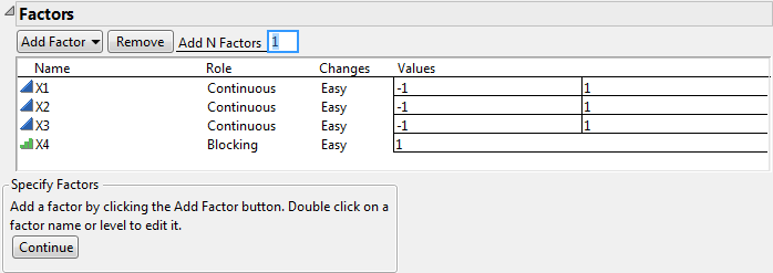
In the Factors outline, type 3 next to Add N Factors.
|
|
3.
|
Click Add Factor > Continuous.
|
|
4.
|
Click Add Factor > Blocking > 3 runs per block.
|
Note that the blocking factor X4 shows only one level under Values. This is because the run size is unknown at this point. Once you click Continue, the Factors outline shows an appropriate number of blocks, calculated as the Default run size divided by the number of runs per block. If you specify a different run size, the Factors outline updates to show the appropriate number of values for the blocking factor.
|
5.
|
Click Continue.
|
The default sample size of 9 requires three blocks. The Factors outline now shows that X4 has three values, indicating the three blocks.
|
6.
|
|
7.
|
In the Model outline, click Interactions > 2nd.
|
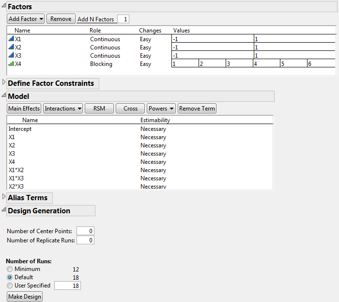
The Number of Runs panel now shows that 18 is the Default run size. Note that the Factors outline has updated to show six values for X4, indicating six blocks.
Note: Setting the Random Seed in step 8 and Number of Starts in step 9 reproduces the exact results shown in this example. In constructing a design on your own, these steps are not necessary.
|
8.
|
(Optional) From the Custom Design red triangle menu, select Set Random Seed, type 458027747, and click OK.
|
|
9.
|
(Optional) From the Custom Design red triangle menu, select Number of Starts, type 10, and click OK.
|
|
10.
|
Click Make Design.
|
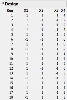
The Design outline shows the design. Recall that X4 is the blocking factor. Observe that the six blocks are represented. When you conduct your experiment, you run the three trials where X4 = 1 on the first day, the three where X4 = 2 on the second day, and so on. So you would like the design table to randomize the trials within blocks. In the Output Options panel, note that Randomize within Blocks is the default setting for Run Order.
|
11.
|
Click Make Table.
|
