Moments

Why are moments important?

Moments are a way to summarize the distribution of a random variable. They have physical interpretations.

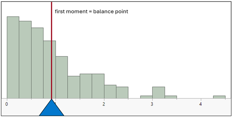
You can think about the first moment, the mean, as the average distance that each point is from zero. The mean is the balance point of the histogram of data, as seen in the figure below.

In physics, the first moment is the sum of force times distance. For example, the first moment of mass is the center of mass. Suppose there are three particles with masses 1 g, 2 g, and 3 g along a line at positions 3 cm, 6 cm, and 8 cm from the origin. The center of mass is, in one dimension, $R_{cw}=\frac{\sum r_i m_i}{\sum m_i}=\frac{3\times1+6\times2+8\times3}{1+2+3}=6.5$ cm.

In statistics, the “force” is the weight of each data value, usually each data value is equally weighted, so the “force” is 1/n, and the “distance” is the data value itself, the distance of the data value from the origin, which is zero. So, the first moment is $\frac{1}{n}\sum_{i=1}^{n} x_i$.

In physics, the second moment is the sum of force squared times distance. For example, the second moment of mass is the moment of inertia. That is, for the masses above, the moment of inertia about the origin is $I=\sum_{i=1}^{n} i\,m_i = 3^2\times1 + 6^2\times2 + 8^2\times3 = 273$.

In statistics, the second raw moment is the average squared distance of each data value from zero. The second raw moment is not as useful in statistics as the second central moment, which is the average squared distance of each data value from the mean. If we only looked at the squared distance of each data value from zero, $\sum_{i=1}^{n} x_i^2$, the moment would include both the spread and the mean of the data. Instead, we remove the effect of the location and look at the squared distance from the mean $\sum_{i=1}^{n}(x_i-\mu)^2$. The second central moment is $\frac{1}{n}\sum_{i=1}^{n}(x_i-\mu)^2$. Subtracting the mean here is analogous to taking the moment of inertia around the center of mass in physics.

The third raw moment is the average cubed distance from zero. The third central moment is the average cubed distance from the mean. Like with the second moment, the cubed distance contains information about both the location and scale of the distribution, so we need to take the average standardized cubed distance around the mean. That is, the third central moment is $\frac{1}{n}\sum_{i=1}^{n}\left(\frac{x_i-\mu}{\sigma}\right)^3$.

The fourth raw moment is the average quartic distance from zero. Again, we need to standardize the data to remove the information about the location and scale. The fourth central moment is $\frac{1}{n}\sum_{i=1}^{n}\left(\frac{x_i-\mu}{\sigma}\right)^4$.

These definitions assume that the population mean $\mu$ and standard deviation $\sigma$ are known. The formulas above will need to be adjusted when we estimate $\mu$ and $\sigma$ with $\bar{x}$ and $s$.

Estimating moments

The first sample moment is simply the sample mean $m_1=\bar{x}=\frac{1}{n}\sum_{i=1}^{n}x_i$. It is an unbiased estimator of the first population moment.

The second sample moment is $m_2=\frac{1}{n}\sum_{i=1}^{n}(x_i-\bar{x})^2$. It is a biased estimator of the population variance $\sigma^2$. The bias is known, and an unbiased estimator of $\sigma^2$ is the sample variance $s^2=\frac{1}{n-1}\sum_{i=1}^{n}(x_i-\bar{x})^2$.

The third sample central moment is $m_3=\frac{1}{n}\sum_{i=1}^{n}(x_i-\bar{x})^3$. It is a biased estimator of the third population central moment. The unbiased sample skewness is given by $\frac{n}{(n-1)(n-2)}\sum_{i=1}^{n}\left(\frac{x_i-\bar{x}}{s}\right)^3$, where s is the sample standard deviation.

The fourth sample central moment is $m_4=\frac{1}{n}\sum_{i=1}^{n}(x_i-\bar{x})^4$. It is a biased estimator of the fourth population central moment. The unbiased sample excess kurtosis is given by $\frac{n(n+1)}{(n-1)(n-2)(n-3)}\sum_{i=1}^{n}\left(\frac{x_i-\bar{x}}{s}\right)^4-\frac{3(n-1)^2}{(n-2)(n-3)}$. Notice that as $n$ $\rightarrow$ $\infty$, the limit of the extra term is 3.

Fitting a distribution using sample moments

The method of moments is used to estimate parameters of a statistical model. To use this method, equate the first sample moment to the first population moment, then equate the second sample moment to the second population moment, and so on until you have the same number of equations as parameters you want to estimate. Finally, solve these equations for the parameters.

For example, suppose you have a sample of data from a beta distribution with unknown parameters $\alpha$ and $\beta$. You’d like to estimate $\alpha$ and $\beta$ from the sample. The mean of the beta distribution is $\frac{\alpha}{\alpha+\beta}$, and the variance is $\frac{\alpha\beta}{(\alpha+\beta)^2(\alpha+\beta+1)}$. We can equate the sample moments, $\bar{x}$ and $s^2$, to these expressions, then solve for $\alpha$ and $\beta$.

$\bar{x}=\frac{\alpha}{\alpha+\beta}$

$s^2=\frac{\alpha\beta}{(\alpha+\beta)^2(\alpha+\beta+1)}$

Solve the first equation for $\beta$:

$\bar{x}(\alpha+\beta)=\alpha$

$\beta\bar{x}=\alpha-\alpha\bar{x}$

$\beta=\frac{\alpha}{\bar{x}}-\alpha$

$\beta=\alpha\left(\frac{1}{\bar{x}}-1\right)$

Next, let $q=\frac{1}{\bar{x}}-1$, then plug in the value for $\beta$ into the second equation and solve for $\alpha$:

$s^2=\frac{\alpha\times\alpha q}{(\alpha+\alpha q)^2(\alpha+\alpha q+1)}$

$=\frac{q}{(1+q)^2(\alpha(1+q)+1)}$

$=\frac{q}{\alpha(1+q)^3+(1+q)^2}$

So $q=s^2\left[\alpha(1+q)^3+(1+q)^2\right]$. Also, $1+q=\frac{1}{\bar{x}}$ and $q=\frac{(1-\bar{x})}{\bar{x}}$, so we can substitute to obtain:

$\frac{1-\bar{x}}{\bar{x}}=s^2\left[\frac{\alpha}{\bar{x}^3}+\frac{1}{\bar{x}^2}\right]$

$\frac{1-\bar{x}}{\bar{x}\times s^2}=\frac{\alpha}{\bar{x}^3}+\frac{1}{\bar{x}^2}$

$\frac{\bar{x}^3(1-\bar{x})}{\bar{x}\times s^2}=\alpha+\bar{x}$

$\hat{\alpha}=\bar{x}\left(\frac{\bar{x}(1-\bar{x})}{s^2}-1\right)$

Substituting in the equation for $\beta$ gives

$\hat{\beta}=\bar{x}\left(\frac{\bar{x}(1-\bar{x})}{s^2}-1\right)\left(\frac{1-\bar{x}}{\bar{x}}\right)$

$\hat{\beta}=(1-\bar{x})\left(\frac{\bar{x}(1-\bar{x})}{s^2}-1\right)$

$\hat{\alpha}$ and $\hat{\beta}$ are the method of moments estimators of $\alpha$ and $\beta$.

The moment ratio diagram

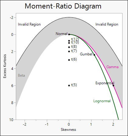
A moment ratio diagram plots kurtosis by skewness for different probability distributions. The diagram can help practitioners characterize data by determining some potential distributions to consider when fitting.

In the moment ratio diagram below, there is an invalid region. No probability distribution can have this combination of skewness and kurtosis. For one-parameter distributions like the t, normal, exponential, or Gumbel, there is one point on the diagram. For some two-parameter distributions, like the lognormal or gamma, there is a curve. The beta distribution has an entire region. You can find a member of the Johnson family of distributions that has any valid combination of skewness and kurtosis.