Exponential Distribution
What is the exponential distribution?
The exponential distribution is a continuous probability distribution that describes the amount of time until an event occurs. It is commonly used to model waiting times between events that occur randomly and independently at a constant average rate. The parameter $\lambda$ (lambda) represents the event rate, sometimes called the failure rate. The exponential distribution is commonly used in reliability analysis.
What are some examples of the exponential distribution?
Examples of the exponential distribution include:
- The time between failures of electronic components or systems.
- The time between customer service calls arriving at a call center.
- The length of a customer service call.
- The time between patient arrivals at an urgent care center.
When should I consider using the exponential distribution?
The exponential distribution is useful for modeling the time until an event occurs when the event rate remains constant over time. In reliability applications, it is often used when failures occur randomly; that is, the reliability of the product is neither improving nor degrading with age. For example, the lifetime of an electronic component is determined by random failures. You might collect failure times from many components and use an exponential model to estimate the probability that a future component survives for a specified amount of time.
The failure rate is the number of failures expected in an interval of fixed length. It’s important to report the length of the interval when specifying the exponential distribution. For example, the failure rate of an electronic component might be 1 per 1,000 hours. This rate is equivalent to 5 per 5,000 hours or 1 per 41.67 days. The mean of the exponential random variable is the reciprocal of the failure rate. That is, if the failure rate is 1 per 1,000 hours, the mean time between failures is 1,000 hours.
You might want to model exponential failure times, like comparing failure rates across products or use conditions. Reliability models, generalized linear models, and penalized regression models can all handle an exponential response variable.
Characteristics of the exponential distribution
The exponential distribution is a special case of the Gamma, Weibull, Chi-square, and F distributions, and it is the continuous analog to the geometric distribution. The exponential distribution measures time until an event occurs, while the geometric distribution counts trials until the first success.
The exponential distribution is closely related to the Poisson distribution. If events occur according to a Poisson process with a constant average rate $\lambda$, then the number of events in a fixed interval follows a Poisson distribution, while the time between consecutive events follows an exponential distribution with the same rate parameter. In this way, the Poisson distribution models event counts, and the exponential distribution models waiting times.
One unique feature of the exponential distribution is its memoryless property. If an item has already survived for a certain amount of time, the probability that it survives additional time does not depend on how long it has already survived. The exponential distribution is the only continuous distribution with this property.
The memoryless property of the exponential distribution leads to a constant hazard function. The hazard function is the instantaneous failure rate over time. This failure rate does not change over time for the exponential distribution. in other words, the failure rate neither increases nor decreases over time. If your process does not have a constant failure rate, consider other reliability distributions like the Weibull distribution or lognormal distribution.
| Model parameters | $\lambda$, the event or failure rate |
| Density function | $f(x) = \lambda e^{-\lambda x}, \; x \geq 0$ |
| Mean | 1 / $\lambda$ |
| Variance | 1 / $\lambda^2$ |
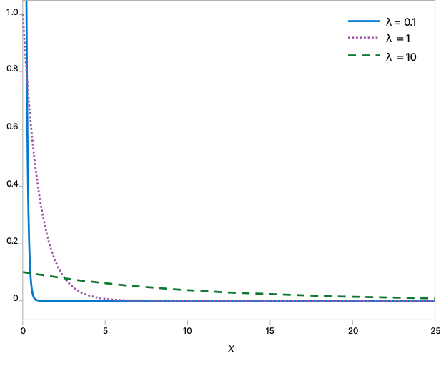
The exponential probability density functions for several values of $\lambda$ are plotted below.
Example of an exponential random variable
Suppose time to failure of a component is given by a random variable $X$. Assume the distribution of $X$ is exponential with parameter $\lambda$. Then the reliability at time $t$ is given by
$R(t) = P(X > t) = \int_t^{\infty} f(x)\,dx = \int_t^{\infty} \lambda e^{-\lambda x}\,dx = e^{-\lambda t}$
For example, if the failure rate for the component is 1 per 100 hours, then the reliability at 200 hours is
$R(200) = e^{-0.01 \cdot 200} = e^{-2} = 0.14$.
That is, there is a 14% chance that the component will survive at least 200 hours.
What is the value of $t$ that would yield a reliability of 95%? We solve $0.95 = e^{-t/100}$, for $t$, yielding $t$ = 5.13 hours.
What value of the failure rate would yield a 95% reliability at 100 hours? We solve $R(t) = e^{-t/100} = 0.95$ for $\lambda$, yielding $\lambda$ = 0.00051 per hour.