Weibull Distribution
What is the Weibull distribution?
The Weibull distribution is a continuous probability distribution that describes the time until an event occurs, often the time until a product, part, or system fails. It is commonly used in reliability analysis because it can model failure rates that decrease, stay constant, or increase over time. This flexibility makes it useful for studying many types of mechanical systems, materials, and lifetime data.
What are some examples of the Weibull distribution?
Examples of the Weibull distribution include:
- The lifetime of a mechanical system with many possible failure points.
- The amount of time a visitor spends on a web page before clicking away.
- Extreme events, such as the largest rainfall total recorded each year.
- Particle sizes in a manufactured material.
- The strength of materials before they break.
When should I consider using the Weibull distribution?
The Weibull distribution is useful when modeling lifetime, failure-time, or time-to-event data, especially when the failure rate might change as time passes. For example, early failures might become less likely after weak parts fail, or failures might become more likely as parts wear out.
You could collect failure times from many units and use a Weibull model to estimate reliability at a future time. You might compare reliability across products, materials, or use conditions. You might also model the Weibull data (often time to failure or time to event data) as a function of independent variables, as in penalized regression.
Other reliability distributions, such as the exponential distribution or lognormal distribution, can be considered when the requirements for the Weibull distribution are not met.
Characteristics of the Weibull distribution
One reason the Weibull distribution is popular in reliability analysis is that it can represent different patterns of failure over time. It is especially useful for “weakest link” situations, where a system can fail when one of many possible parts or mechanisms fails first.
The Weibull distribution has two parameters: the shape, $\beta$, and scale, $\alpha$. (In some parameterizations, these are the location, $\mu$, and scale, $\sigma$, as shown in the table below.) The shape parameter $\beta$ describes how the failure rate changes over time. In practice, the shape parameter is often the most important part of the Weibull distribution. It tells whether failures happen mostly early, at a roughly constant rate, or increasingly often as items age. The scale parameter $\alpha$ is often called the characteristic life.
A useful special case occurs when the shape parameter $\beta$ = 1. In that case, the Weibull distribution is the exponential distribution.
| Model parameters | $\beta$ the shape, $\beta$ = 1/$\sigma$ $\alpha$, the scale, or characteristic life (or 63.2% quantile, $\alpha = e^\mu$) or $\mu$, the location, $\mu$ = log($\alpha$) $\sigma$, the scale, $\sigma$ = 1/$\beta$ |
| Mass function | $f(x) = \frac{\beta}{\alpha}\left(\frac{x}{\alpha}\right)^{\beta-1} e^{-\left(\frac{x}{\alpha}\right)^{\beta}}, \; x > 0,\; \alpha > 0,\; \beta > 0$ |
| Mean | $\alpha \Gamma\!\left(1+\frac{1}{\beta}\right)$ |
| Variance | $\alpha^2 \left[ \Gamma\!\left(1+\frac{2}{\beta}\right) - \Gamma^2\!\left(1+\frac{1}{\beta}\right) \right]$ |
The graph below shows Weibull density functions for several different $\beta$s with the same $\alpha$.
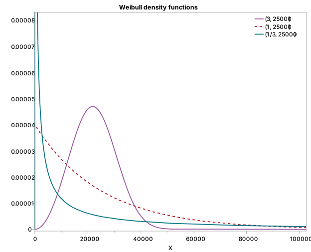
More formally, the shape parameter $\beta$ determines the shape of the hazard function, or failure rate over time. The graph below shows the hazard function for the same density functions in the previous graph.
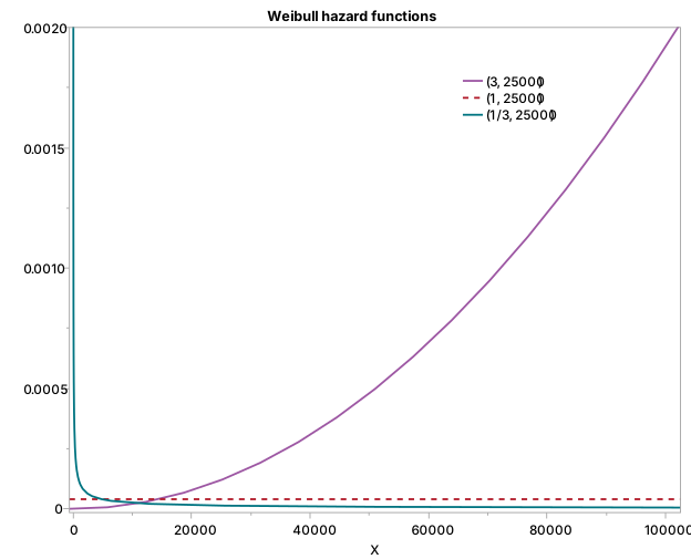
If $\beta$ = 1 (that is, the Weibull distribution is the exponential distribution), the hazard is constant. If $\beta$ < 1, the hazard decreases over time, which can describe early failures that become less likely after the weakest units fail. If $\beta$ > 1, the hazard increases over time, which can describe wear-out failures where older units are more likely to fail.
Example of a Weibull random variable
Suppose a population of capacitors follows a Weibull distribution with characteristic life $\alpha$ = 25,000 hours and shape parameter $\beta$ = 0.5. What is the probability that a new capacitor fails by 1,000 hours?
$P(T < 1000) = \int_{0}^{1000} f(t)\,dt = \int_{0}^{1000} \frac{0.5}{25000}\left(\frac{t}{25000}\right)^{0.5-1} e^{-\left(\frac{t}{25000}\right)^{0.5}}\,dt = 0.18$
The probability of failure by 1,000 hours is 18%, so the reliability at 1,000 hours is 82%. At the characteristic life (25,000 hours), the probability of failure is 63.2%. This is why the scale parameter $\alpha$ is also called the 63.2% quantile.
Now suppose the characteristic life stays the same, but the shape parameter changes to $\beta$ = 2. The probability of failure by 1,000 hours is only 0.16%, but the probability of failure by 25,000 hours is still 63.2%. The shape parameter changes how quickly failures accumulate before and after the characteristic life, but it does not change the meaning of the characteristic life itself.