Poisson Distribution
What is the Poisson distribution?
The Poisson distribution is a discrete probability distribution for count data. It describes the probability of seeing a given number of events in a fixed amount of time or space. A process where events occur independently and at a constant average rate is called a Poisson process. The Poisson distribution parameter $\lambda$ (lambda) describes the rate, which is the expected number of events in the interval you are studying.
What are some examples of the Poisson distribution?
The Poisson distribution arises in diverse situations. Examples include:
- The number of buses that arrive at a bus stop in 30 minutes.
- The number of customers who enter a store in one hour.
- The number of earthquakes occurring in a specific region over a year.
- The number of defects in a square yard of carpet.
- The number of patients arriving at the emergency room during a shift.
When should I consider using the Poisson distribution?
The Poisson distribution is useful when you are counting how many times an event occurs in a fixed interval. The interval might be a period of time, such as one hour, or a fixed amount of space, such as one square yard. The average rate of events must be constant across that interval. You can estimate the average number of events per interval by dividing the number of events counted by the desired interval. For example, if you observe a bus stop for 50 hours and count 100 buses, you would estimate the rate as $\lambda$ = 100 / 50 = 2 buses per hour.
In a Poisson process, the expected number of events in an interval of fixed length depends only on the length of the interval and not on how long it has been since the last event. For example, imagine a city where buses arrive randomly rather than on a fixed schedule. The number of buses arriving in a 30-minute interval might follow a Poisson distribution. In that scenario, the probability that a bus arrives in the next 30 minutes does not depend on how long you’ve already been waiting! It’s the same whether you’ve been waiting for two hours or two minutes.
The interval over which you count events is sometimes called the area of opportunity. In the bus example, the area of opportunity is 30 minutes. The parameter $\lambda$ represents the average number of buses that arrive during that 30-minute interval. You can change the interval as long as you also adjust the rate to match. For example, a rate of two buses per 30 minutes is the same as four buses per hour or one bus per 15 minutes. When comparing Poisson counts, make sure the counts are based on the same interval. Comparing 30-minute counts in one city with 60-minute counts in another city would not be a fair comparison.
You might want to model Poisson counts as a function of independent variables, like comparing bus arrivals across different cities or on different routes within a city. Generalized linear models and penalized regression models are well-suited for scenarios like this.
Characteristics of the Poisson distribution
A key feature of the Poisson distribution is that its mean and variance are equal. However, in practice, count data sometimes exhibit more variability than is expected under the Poisson distribution; that is, the variance is greater than the mean. This is referred to as overdispersion. When count data are overdispersed, the negative binomial distribution can be used to model the data. In fact, the Poisson distribution is a special case of the negative binomial.
The Poisson distribution is closely related to the exponential distribution. The Poisson distribution counts how many events occur in a fixed interval. The exponential distribution measures the time between events in a Poisson process. In other words, the Poisson distribution models event counts, while the exponential distribution models waiting times. The likelihood of the Poisson probability only depending on the length of the interval (or size of the space) is directly related to the memoryless property of the exponential distribution.
| Model parameters | $\lambda$, the rate of events per unit time or space |
| Mass function | $p(x) = \frac{e^{-\lambda}\lambda^x}{x!}, \; x = 0,1,2,\ldots$ |
| Mean | $\lambda$ |
| Variance | $\lambda$ |
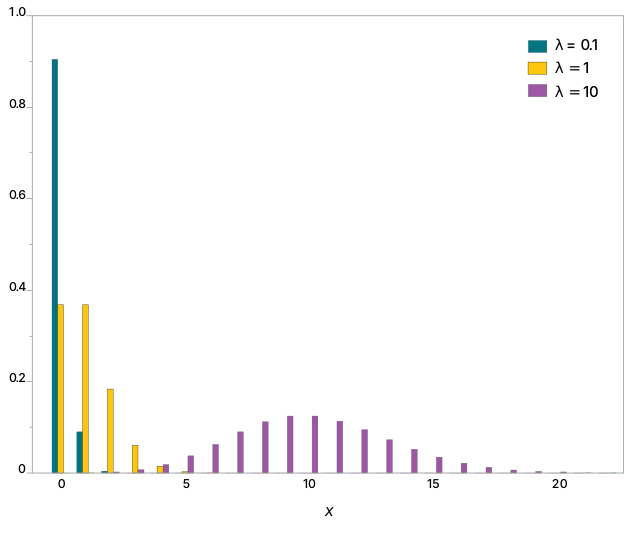
The graph below shows the Poisson probability mass function for $\lambda$ = 0.1, $\lambda$ = 1, and $\lambda$ = 10.
Example of a Poisson random variable
Suppose demand for a certain car part at an automotive parts store occurs randomly, with an average rate of one order every five years. The store owner wants to estimate the probability that the part will be ordered in the next year, the next six months, or the next month. If t is the number of years in the time period, then the number of orders in the next t years follows a Poisson distribution with parameter $\lambda$ = 1/5 x t.
To find the probability that the part will be ordered in the next year, it is easiest to first find the probability that the part will not be ordered, then subtract that value from 1.
$P(X > 0) = 1 - P(X = 0) = 1 - e^{-\lambda} = 1 - e^{-0.2} = 0.18$
There is about an 18% chance that the part will be ordered in the next year.
For the probability that the part will be ordered in the next six months, the time period is one-half year, so the Poisson parameter is $\lambda$ = 1/5 x 1/2 = 0.1.
$P(X > 0) = 1 - P(X = 0) = 1 - e^{-\lambda} = 1 - e^{-0.1} = 0.095$
There is about a 10% chance that the part will be ordered in the next six months.
Finally, for the probability that the part will be ordered in the next month, the time period is one-twelfth of a year, so the Poisson parameter is $\lambda$ = 1/5 x 1/12 = 0.0167.
$P(X > 0) = 1 - P(X = 0) = 1 - e^{-\lambda} = 1 - e^{-0.0167} = 0.0165$
The chance that the part will be ordered in the next month is less than 2%.