Negative Binomial Distribution
What is the negative binomial distribution?
The negative binomial distribution is a discrete probability distribution that describes how many failures occur before a fixed number of successes in independent Bernoulli trials. Each trial has only two possible outcomes: success or failure. The probability of success in each trial is $p$. The fixed number of successes is often written as $k$.
What are some examples of the negative binomial distribution?
Examples of the negative binomial distribution include:
- The number of missed free throws before a basketball player makes three successful shots.
- The number of defective items produced before a process produces 10 non-defective items.
- The number of job applications reviewed before finding five qualified applicants.
- The number of sales calls made before closing a specified number of sales.
When should I consider using the negative binomial distribution?
The negative binomial distribution is useful when the number of successes is fixed, but the number of trials or failures needed to reach that number is random. The trials must be independent, and the probability of success is the same in each trial.
You might also use the negative binomial distribution to model count data when the variance is larger than the mean. This situation can occur if the successes are clustered together in space or time, and is called overdispersion (variance is a measure of dispersion). A Poisson distribution assumes that the mean and variance are equal, so the negative binomial distribution is often used when a Poisson model does not allow the observed variability.
Characteristics of the negative binomial distribution
The negative binomial distribution is a generalization of the geometric distribution. The geometric distribution models the number of failures before the first success; the negative binomial models the number of failures before the $k$th success.
This distribution is sometimes described as a gamma-Poisson distribution. In that version, the count follows a Poisson distribution, but the Poisson rate is not fixed; it varies according to a gamma distribution. It is similar to how the beta binomial distribution extends the binomial distribution by allowing the probability of success to vary.
| Model parameters | $k$, how many successes, $k$ = 0, 1, 2, ... $p$, the probability of success on each trial |
| Mass function | $p(X=x)=\binom{x+k-1}{x}p^{k}(1-p)^{x},\quad x=0,1,2,\ldots$ |
| Mean | $k$($1-p$) / $p$ |
| Variance | $k$($1-p$) / $p^2$ |
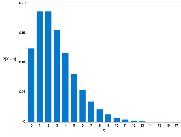
The graph below shows a negative binomial distribution when k = 3 and p = 0.5.
Why is it called the negative binomial distribution?
The name comes from a mathematical connection to the binomial theorem. The probability mass function can be written using a coefficient with a negative upper term, sometimes called a negative binomial coefficient:
$p(X=x)=\binom{-k}{x}p^{k}\bigl(-(1-p)\bigr)^{x},\quad x=0,1,2,\ldots$
This more advanced form also allows the success parameter $k$ to be extended beyond positive integers in some settings.
Example of a negative binomial random variable
In a golf skills challenge, a competitor must hit a target three times before moving to the next stage. Suppose the probability of hitting the target on each attempt is 0.5. What is the probability that the competitor completes the challenge in five attempts or fewer?
Completing the challenge in five attempts or fewer means having 0, 1, or 2 failures before the third success. Let $x$ be the number of failures before the third success. Then $x$ follows a negative binomial distribution with $k$ = 3 and $p$ = 0.5.
\[ \begin{aligned} P(X \le 2) &=\sum_{x=0}^{2}\binom{x+3-1}{x}(0.5)^{3+x} \\ &=\binom{2}{0}0.5^3+\binom{3}{1}0.5^4+\binom{4}{2}0.5^5 \\ &=0.125+3\times0.0625+6\times0.03125 \\ &=0.5 \end{aligned} \]
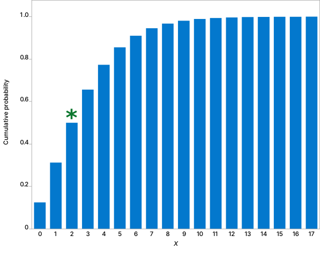
The probability of completing the challenge in five attempts or fewer is 50%, indicated by the asterisk in the graph below.