Geometric Distribution
What is the geometric distribution?
The geometric distribution is a discrete probability distribution that describes how many independent Bernoulli trials occur before the first success. Each trial has only two possible outcomes (success or failure), and the probability of success in each trial is $p$. The geometric distribution is a special case of the negative binomial distribution when you are only interested in the number of trials until the first success.
What are some examples of the geometric distribution?
Examples of the geometric distribution include:
- The number of coin flips until the coin comes up heads.
- The number of pulls on the pull cord before a lawnmower starts.
- The number of throws attempted before making a bullseye in the game of darts.
- The number of items from an assembly line inspected until a defective item is found.
When should I consider using the geometric distribution?
The geometric distribution is useful when modeling the number of trials until first success. You might collect data from multiple scenarios and estimate $p$, the probability of success.
As mentioned above, the geometric distribution is a special case of the negative binomial distribution. In the geometric distribution, the number of successes is 1; in other words, you are only interested in how many trials occur before a single success. The negative binomial distribution models the number of trials until the $k$th success (where $k \ge 1$).
The geometric distribution is a discrete analog to the exponential distribution. The geometric distribution counts trials until the first success, the exponential distribution measures time until an event occurs.
Characteristics of the geometric distribution
The geometric distribution is a memoryless distribution, meaning that regardless of how many trials have occurred, the probability of success in future trials doesn’t change. For example, when trying to start your lawnmower by pulling the cord, the probability of needing additional pulls of the cord doesn’t depend on how many times you’ve already pulled it. We write this property as the conditional probability
$P((X > k+t)\mid X > t) = P(X > k)$
That is, it doesn’t matter how many times you pull the lawnmower handle, the probability for future pulls is the same as when you started. This property is directly related to the independence assumption.
Note that the mass function shown below is based on counting the number of trials until the first success. The smallest value the count can take is 1. An alternative version of the geometric distribution counts the number of failures that occur before the first success, so the count could take a value of 0.
| Model parameter | $p$, the probability of success on one trial |
| Mass function | $p(X=x)=p(1-p)^{x-1},\quad x=1,2,3,\ldots$ |
| Mean | $1/p$ |
| Variance | $(1-p) / p^2$ |
Example of a geometric random variable
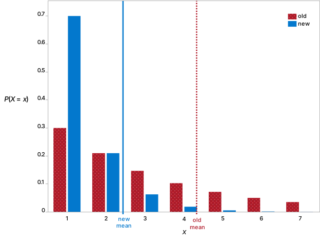
Suppose your old lawnmower had a 30% chance of starting each time you pulled the cord. You purchase a new lawnmower that has a 70% chance of starting with each pull of the cord.
The old lawnmower had an average of $1/p = 1/0.3 = 3.33$ pulls until starting. The new lawnmower has an average of $1/p=1/0.7=1.43$ pulls until starting.
The graph below shows the probabilities of the old and new lawnmowers starting on exactly the $x$th cord pull, along with the mean number of pulls until starting for each mower.