Effect Size
What is effect size?
In statistical hypothesis testing, the effect size is a way to describe how large or meaningful a difference, relationship, or change is. Effect size is one of the five quantities in the calculations for a power analysis.
To determine the effect size that matters to you, consider what change in the response is clinically significant, practically significant, or operationally meaningful.
Why does effect size matter in power analysis?
Power analysis uses effect size to connect the size of an effect you want to detect with the sample size needed to detect it at a given significance level with a high enough probability in the presence of variability. Larger effects are easier to distinguish from natural variation and generally require smaller sample sizes. Smaller effects are harder to detect and generally require larger sample sizes.
Choosing an effect size is often one of the most important parts of planning a study. It should reflect the smallest difference, relationship, or change that would be scientifically, operationally, clinically, or practically meaningful – not merely the largest effect you hope to see.
You can express effect size in the same units as the response variable or in units of the standard deviation of the response variable.
Determining effect size in power analysis
One of the tasks in a power analysis is to specify the effect size for which you are calculating the power. When deciding on which effect size to use, consider the following:
- Minimum difference that matters to you,
- Maximum difference you expect.
- Typical difference you expect.
To elicit a reasonable effect size to use in a power analysis, ask questions like, “What size effect are you looking for?” and “What is the minimum increase that you want?” You can bracket good values for the effect size by asking, “Does an increase of 1, 5, or 10 matter to you?” then increase the sizes until the team responds, “Yes!”
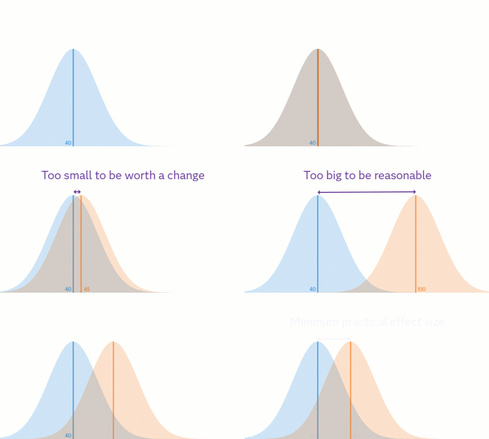
For example, suppose you are part of a team comparing two manufacturing settings. You would like to switch settings if doing so would improve the response. You are ready to run a power analysis to determine a good sample size. What effect size are you interested in? The typical response at the old setting is 40. A change in the typical response from 40 to 45 is not enough to warrant the cost of a process change. A change from 40 to 100 would be terrific, but it’s unreasonable to expect the new process to deliver that much improvement. The team decides that a change from 40 to 60 is reasonable, so you can use 60 – 40 = 20 as the effect size.
In the animation below, you can see the effect size that is too small to be worth a process change, too big to be reasonably expected, and the final determined minimum practical effect size.
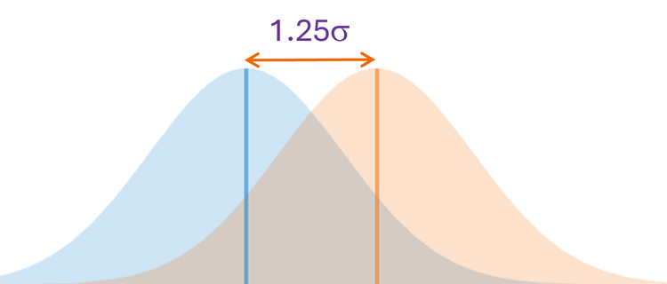
Sometimes it can be easier to work in standard deviation units instead of response units. For example, maybe a 1$\sigma$ difference in means is not enough to warrant a change in the process, but a 2$\sigma$ difference is big enough.
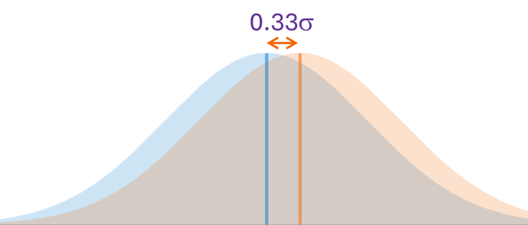
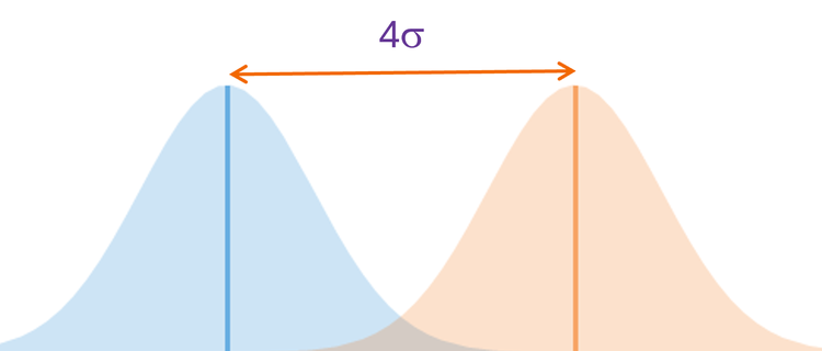
In the example, if the within group standard deviation is 15, then a 20-unit difference in the response is a 1.25$\sigma$ effect. The figures below show the difference that is too small (0.33$\sigma$), too big to be reasonably expected (4$\sigma$), and the minimum practical difference (1.25$\sigma$) in standard deviation units. Of course, your situation will be different. Maybe for your data, 4$\sigma$ is a small effect and 20$\sigma$ is unreasonably large! You will need to use your subject matter knowledge to elicit the desired detectable effect.
Effect size with more than one factor
Understanding power is also important in designing experiments with more than one factor. For example, when screening important factors, you might want to find the relationship between effect size and power for each term in your model (for a given noise variability, sample size, and significance level). Even when you know which factors are important and your goal is optimization, power calculations can be important, for example, when determining how many patients to enroll in a medical study.
Suppose you have two continuous factors, each at two levels, and you would like to raise your response from 40 to 60, and your process standard deviation is 15. Since the two levels of the continuous factor values are often coded as –1 and +1, the increase from 40 to 60 is represented by a slope of (60 – 40) / (1 – (–1)) = 20 / 2 = 10.
You might choose to look at the power for each main effect and interaction effect to have a coefficient of 10, which means that the power for each main effect and interaction is for the full effect size. Due to the hierarchy principle, interaction effects are often smaller than main effects, so you might choose to look at the power for each main effect to have a coefficient of 10, and the power for interaction effect to have a coefficient of 5, for example.
Since the intercept in statistical linear models doesn’t often have a physical meaning, you aren’t often interested in testing hypotheses about the intercept.
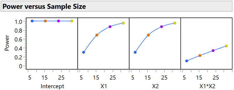
The power for the model terms using a significance level of $\alpha$ = 0.05, noise standard deviation of 15, and coefficients of 10 for the main effects and 5 for the interaction effect, as the total sample size for the experiment changes is shown in the table below. The results can be visualized in the figure below the table. As sample size increases, power increases.
| Term | Anticipated coefficient |
8 runs power |
16 runs power |
24 runs power |
32 runs power |
| Intercept | 50 | 1.000 | 1.000 | 1.000 | 1.000 |
| X1 | 10 | 0.306 | 0.688 | 0.874 | 0.953 |
| X2 | 10 | 0.306 | 0.688 | 0.874 | 0.953 |
| X1 x X2 | 5 | 0.114 | 0.233 | 0.343 | 0.445 |