Multiple Comparisons
What are multiple comparisons?
A multiple comparison test is a hypothesis test that is used to determine which groups have different means in a one-way ANOVA. If the F test of the one-way ANOVA is statistically significant, the null hypothesis of equal means is rejected. However, the F test can’t tell you which group means are different. A multiple comparison test identifies which group means are different from each other. A multiple comparison test controls the experiment-wise error rate instead of the comparison-wise error rate.
You can think of experiment-wise and comparison-wise error rates by using the following example. Suppose you are planning a road trip in your old car and the probability of failure of a key engine component is 5%. You might be willing to leave on your trip in this car if you had a 5% chance of engine failure over the duration of the trip. Now suppose there were 10 key components in the engine, each with a 5% change of failure during the trip. The overall chance of engine failure (assuming independent failures) is about 90%. You probably wouldn’t be willing to leave on your trip in this car! In multiple comparisons, the chance of one component failing is like testing the difference between a pair of group means. The chance of at least one component failing over the whole group of components is like testing the difference between all possible pairs of group means.
Making multiple comparisons such as comparing pairs of means using one-way ANOVA increases the possibility of declaring a difference significant when there is not a real difference in the group means. We are satisfied with a 100$\alpha$% chance of committing this type of error, where $\alpha$ is chosen by the researcher. However, the more tests you do, the more likely you are to happen upon a significant difference occurring by chance alone. If you compare all possible means in a one-way layout with many different levels, there are many possible tests, and calling a difference significant, when in reality it is not, becomes very likely.
Recall the hypotheses for the ANOVA F test:
$H_0$: all group means equal
$H_1$: not all group means equal
Rejecting the null hypothesis $H_0$ enables you to conclude that at least one mean is different from the others. It does not inform you about which group means are different. Comparing many pairs of means to each other introduces the problem of multiple comparisons.
Suppose you are using a significance level of $\alpha$ = 0.05 and your ANOVA F test is significant. You then want to know which group means are different. If you compare all means to each other using a two-samplet-test for each comparison, you have a probability of not making an error of 1 – $\alpha$ = 1 – 0.05 = 0.95 for each comparison. The probability of not making an error when the null hypothesis is true among all $n$ comparisons is $0.95^n$. This probability is called the experiment-wise error rate. The significance level is the comparison-wise error rate.
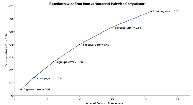
The figure above displays the experiment-wise error rate, that is, the probability of committing at least one Type I error when comparing all pairs of group means by the number of comparisons at $\alpha$ = 0.05. The number of comparisons made is the number of ways to choose two group means from all the group means, that is $\binom{k}{2}=\frac{k!}{2!(k-2)!}=\frac{k(k-1)}{2}$ where $k$ is the number of groups. For example, for two groups, there is just one comparison. For three groups, there are three comparisons. For seven groups, there are 21 comparisons. Even though the comparison-wise error rate stays the same at 5%, the experiment-wise error rate – that is, the probability of at least one Type I error in all the tests – increases as the number of comparisons increases.
Multiple comparison tests
There are many different multiple comparison methods available in statistical software. They can be compared based on the number of comparisons to be made and the adjustment to the $\alpha$ level.
The table below summarizes many of these tests, ranked approximately from least conservative to most.
| Procedure | Control | Number of comparisons | Use |
| Student t | Comparison-wise | (k – 1) / 2 | Single comparison |
| Student-Newman-Keuls | Stepwise | varies | All comparisons |
| Fieller | Experiment-wise | k(k – 1) / 2 | Tests ratios of group means, equal or unequal variances |
| Hsu MCB | Experiment-wise | k – 1 | Compare with min or max |
| Dunnett | Experiment-wise | k – 1 | Compare to control group |
| Tukey-Kramer | Experiment-wise | k(k – 1) / 2 | All comparisons |
| Games-Howell | Experiment-wise | k(k – 1) / 2 | All comparisons, unequal sample sizes, unequal variances |
| Bonferroni | Experiment-wise | k(k – 1) / 2 | All comparisons |
- The Student t-test approach, also known as Fisher’s least significant difference (LSD), controls only the comparison-wise error rate, and the other approaches control the experiment-wise error rate.
- The Student-Newman-Keuls test is an iterative procedure that orders the group means, then compares the largest and smallest means. If a significant difference is found, the procedure compares the groups with the next largest difference in group means, and so on. If a comparison results in no significant difference being found, the comparisons end and all other differences are deemed non-significant. This procedure controls the experiment-wise error rate under the complete null hypothesis but does not control the maximum experiment-wise error rate under any partial null hypothesis. That is, it allows more Type I errors in individual comparisons but has higher power and might be more beneficial when Type II errors are a larger concern than Type I errors and you have many groups.
- Fieller compares ratios of group means instead of differences of group means. This method can be useful when the ratio matters more than the difference, for example, in comparing gene expression in groups by comparing fluorescence to a standard.
- Hsu’s MCB (multiple comparison with best) test is similar to Dunnett’s but compares to the group with the sample minimum or maximum instead of a control group.
- Dunnett’s test is a special case that compares each group only to a control group. The groups are not compared to each other, only to a control. The total number of comparisons is reduced, so the adjustment to $\alpha$ is smaller than the adjustment in the Tukey-Kramer test.
- The Tukey-Kramer method, also known as the Tukey honestly significant difference (HSD) test, controls the experiment-wise error rate for all pairwise comparisons. It is a good general-purpose multiple comparison test.
- Games-Howell is similar to Tukey-Kramer but uses Welch’s method to adjust for unequal variances if needed.
- A Bonferroni correction uses the Student t approach but modifies the significance level for each comparison so the overall significance level is $\alpha$. Each comparison is performed at $\alpha / nc$, where $nc$ is the number of comparisons.
Example of the Tukey-Kramer multiple comparison test
Suppose you are studying the effect of five different fertilizers on crop yield. You have grown plants in 12 fields per fertilizer and have measured the bushels of crop per acre. The data are shown in the following table.
| None | Urea | Ammonium Sulfate | UAN-32 | Enhanced Efficiency Nitrogen |
| 100.4 | 95 | 104 | 113.4 | 106.7 |
| 99.6 | 101.3 | 105.6 | 111.9 | 104.3 |
| 101.9 | 98.3 | 108.4 | 109.1 | 101.8 |
| 100.3 | 99.8 | 110.5 | 104.4 | 101.2 |
| 98.4 | 100.4 | 102.2 | 108 | 102.6 |
| 101.1 | 101.1 | 110.5 | 110 | 104.7 |
| 103.9 | 103.2 | 110 | 104.1 | 101 |
| 102.8 | 105.1 | 108.3 | 109.2 | 103.4 |
| 97.9 | 101.6 | 106.8 | 109.3 | 103.5 |
| 96.2 | 106.1 | 105.1 | 110.1 | 105.6 |
| 98.1 | 100 | 110.4 | 104.4 | 104.6 |
| 100.1 | 103.1 | 111.9 | 106 |
First, you can graph the data. From the figure below, it appears the assumptions of normality and equal variances within each group are met. The independence assumption is satisfied by the design of the experiment. Treatments were randomly assigned to fields.
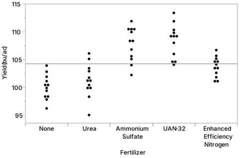
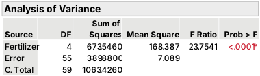
Next, you can fit a one-way ANOVA model to the data. The null hypothesis is that the mean yield is the same for each fertilizer treatment. The alternative is that at least one mean is different from the others. As seen below, the F test has a p-value of less than 0.0001, indicating we should reject the null hypothesis.
Rejecting the null hypothesis tells us that some group means are different from each other. But which ones? From the graph, it looks like None and Urea might have the same mean, and they might have different means than the other three groups. Use a Tukey-Kramer test to answer this question.
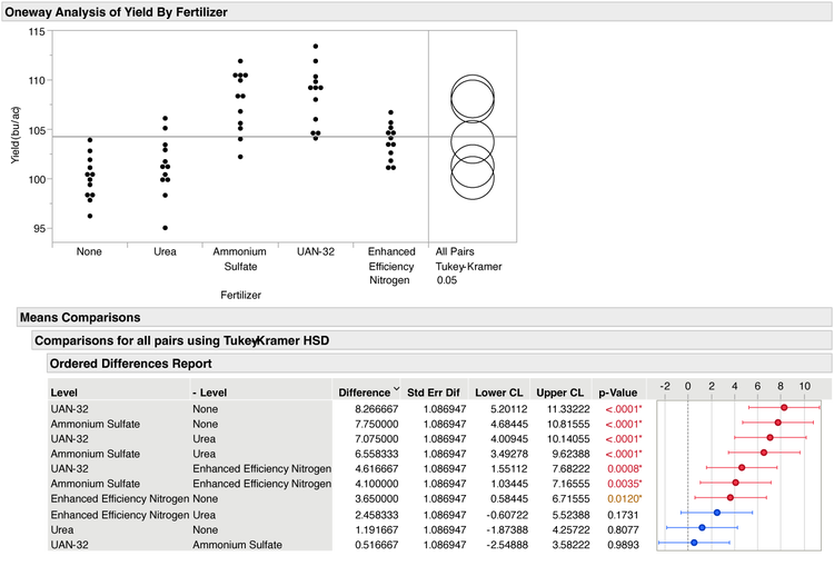
The Ordered Differences Report shows which pairs of means are significantly different from each other. Using an experiment-wise $\alpha$ = 0.05, there are seven significant differences and three non-significant differences.
The circles on the plot are a graphical way of seeing the differences.
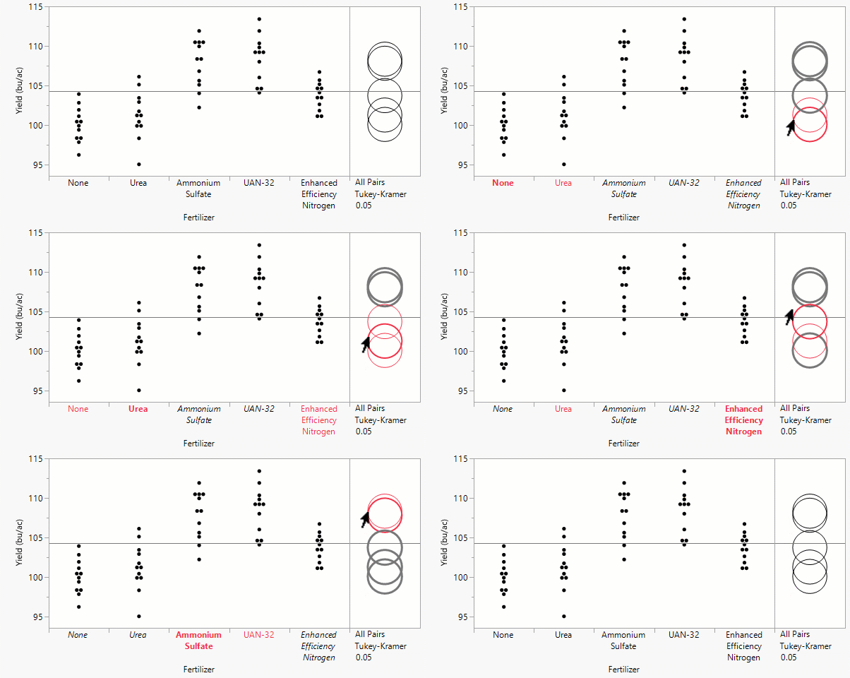
- The mean of the None group is not significantly different from Urea, but it is significantly different from the other three.
- The mean of the Urea group is not significantly different from the None group or the Enhanced Efficiency Nitrogen group, but it is significantly different from Ammonium Sulfate and UAN-32.
- The Ammonium Sulfate group mean is not significantly different from the UAN-32 group mean, but it is significantly different from the other three.
- The UAN-32 group mean is not significantly different from the Ammonium Sulfate group mean, but it is significantly different from the other three.
- The mean of the Enhanced Efficiency Nitrogen group is not significantly different from the mean of the Urea group, but it is significantly different from the other three.
Experiment-wise vs. comparison-wise error rates
What if you had analyzed all 10 comparisons of the fertilizer group means using two-sample t-tests – in other words, incorrectly not doing any adjustment for the multiple comparisons?
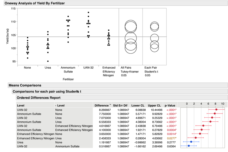
You would have found more statistically significant differences! Controlling each comparison at $\alpha$ = 0.05 instead of all comparisons at $\alpha$ = 0.05 finds that there is an additional significant difference in the means between Urea and Enhanced Efficiency Nitrogen. There is a higher probability of a false alarm (making a Type I error) when finding differences in means using all two-sample t-tests. A multiple comparison test controls the experiment-wise error rate instead of the comparison-wise error rate.