Importing Series Matrix Files

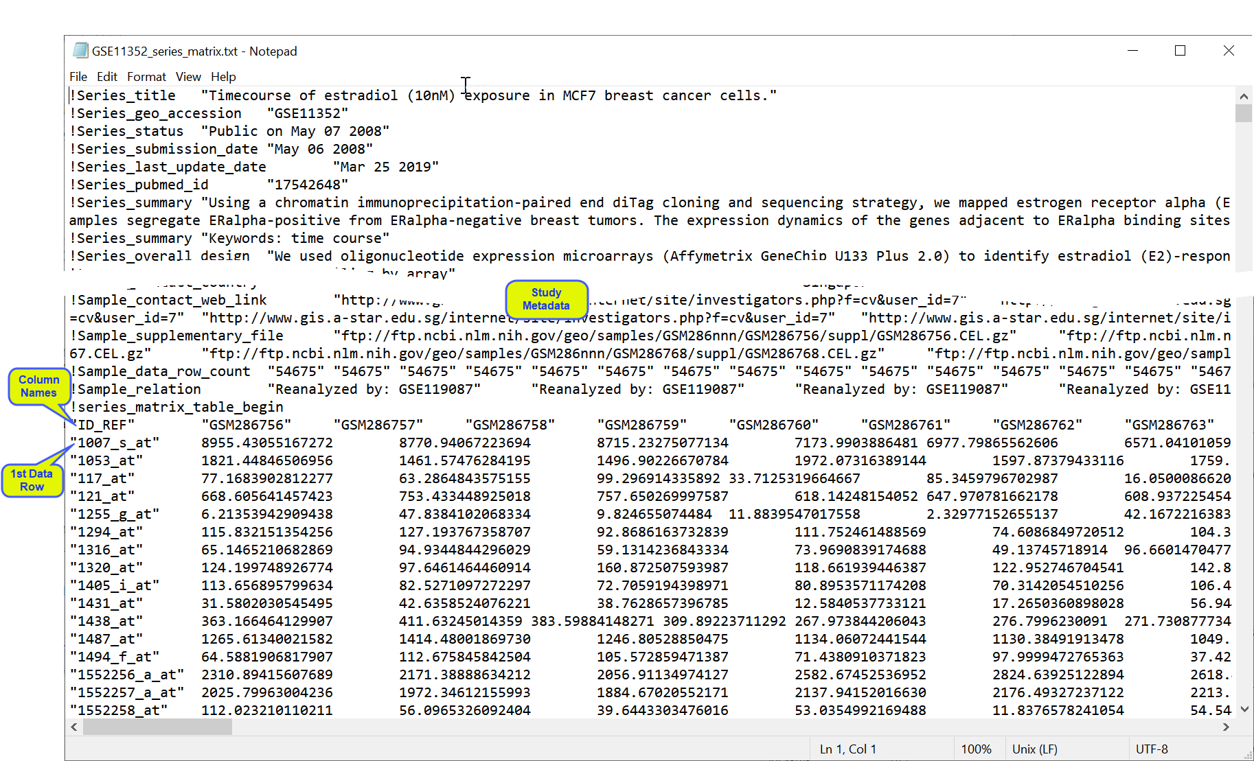
Series matrix files are text files that include a tab-delimited matrix generated from the VALUE column of each sample. The matrix is headed with multiple rows, prefaced with an exclamation point (!) listing sample and series metadata. A row listing the column names for the matrix follows directly after the metadata. This row is followed, in turn, by the data. Genes in are rows with each sample comprising a column (Tall format A data table in which variables in rows and samples are in the columns). The GSE11352 series matrix, used in this example, is freely available from the Gene Expression Omnibus (GEO), and is shown below.

Importing Series Matrix Files into JMP PRO

In this example, we import the files shown above.

Select File > Open. An Open Data File window opens to the last location used.

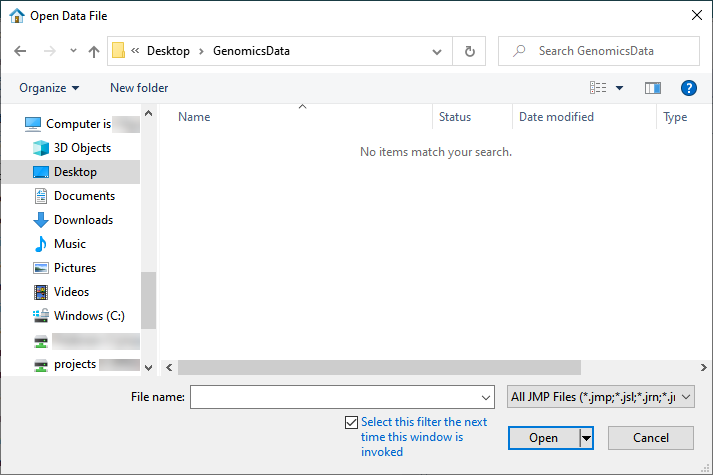
Navigate to the location of the txt file and use the drop-down menu (shown below) to select All Files (*.*).

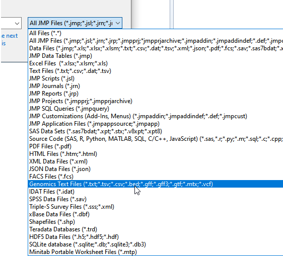
The options in the window change.

Select the desired file.

Check the Open as Data (Using Preview) radio button.

Click .

The Preview window is shown below:

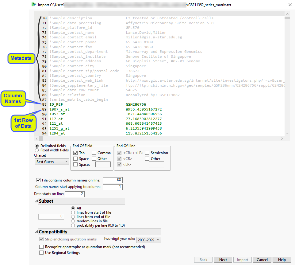
The preview enables you to visually inspect your data. You can identify the rows containing metadata and column names. Scroll through the table to determine the rows and columns containing the data. In this example, all of the content to be imported into the JMP table is shown in black. This includes the row of column names (row 25) and all of the data starting with row 26). Vertical bars in the table delimit the data included in each column.

Examine the preview. Content not contained in the column name and data rows are grayed out and are not included in the JMP table.

The wizard also presents options for specifying features of and subsetting the data. Refer to Options in the JMP Text Import Window for more information about these options.In most cases, you will not need to change default settings for these options. However, you might need to specify the rows containing column names and the start of the data. (Note: The line the data starts on refers to the row actually imported.) Additionally, it can be useful to subset very large data sets into multiple JMP tables that can be joined later.

Once you have specified the column name and data rows and any sub-setting options, click .

If everything is satisfactory, click to generate the JMP table.

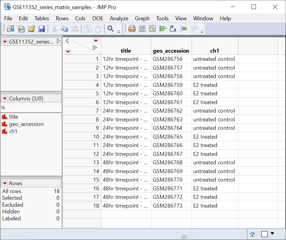
Two tables are generated by the import process: the GSE11352_series_matrix.jmp table containing the experimental data and the GSE11352_series_matrix_samples.jmp table containing information about the design of the experiment.

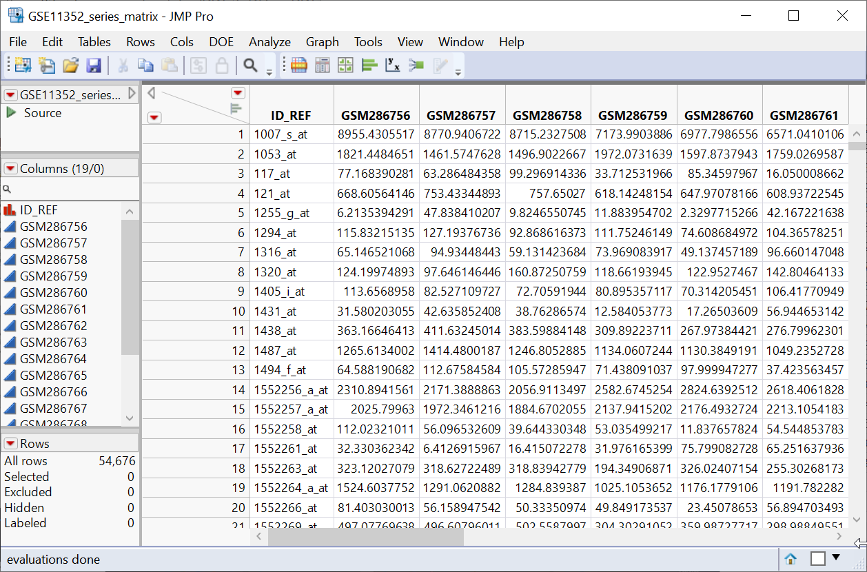
The GSE11352_series_matrix.jmp table contains the data in 18 data columns (+ 1 column with gene

Before we continue, let us discuss how genomic data should be structured for analysis in JMP Pro. Most of the processes in JMP Pro assume that the input table has a particular data structure. JMP Pro distinguishes between tall and wide data sets. A tall data table A data table in which variables in rows and samples are in the columns has samples as columns and molecular entity (for example, markers, genes, clones, proteins, or metabolites) as rows, whereas a wide data table A data table in which variables are columns and samples are rows. is the transpose of the tall, having the samples as rows and molecular entities as columns. The GSE11352_series_matrix.jmp table above is a tall table.

When specifying the input data set for a process, it is important to know the required form. Most genomic analyses in JMP Pro require a wide data table. The Transpose platform under the Tables menu enables you to transform your data tables between tall and wide forms. We will use this option to convert the GSE11352_series_matrix.jmp tall table to a wide format suitable for analysis.

Click on the GSE11352_series_matrix.jmp table to make it active.

Select Tables > Transpose. The Transpose window opens.

The Transpose window was completed as shown below, with the data columns specified as the Transpose Columns, ID_REF as the Label, GSE11352_wide as the Output table name, and geo_accession as the Label column name.

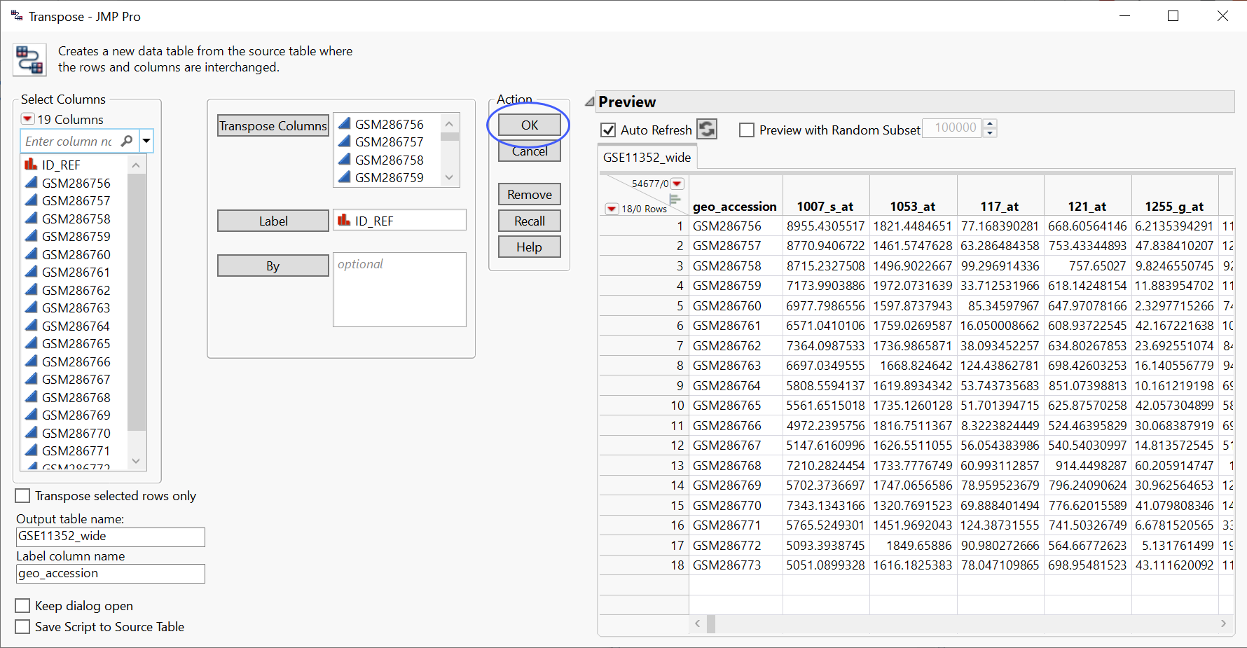
Click to transpose the table.

The resulting GSE11352_wide table is shown below.

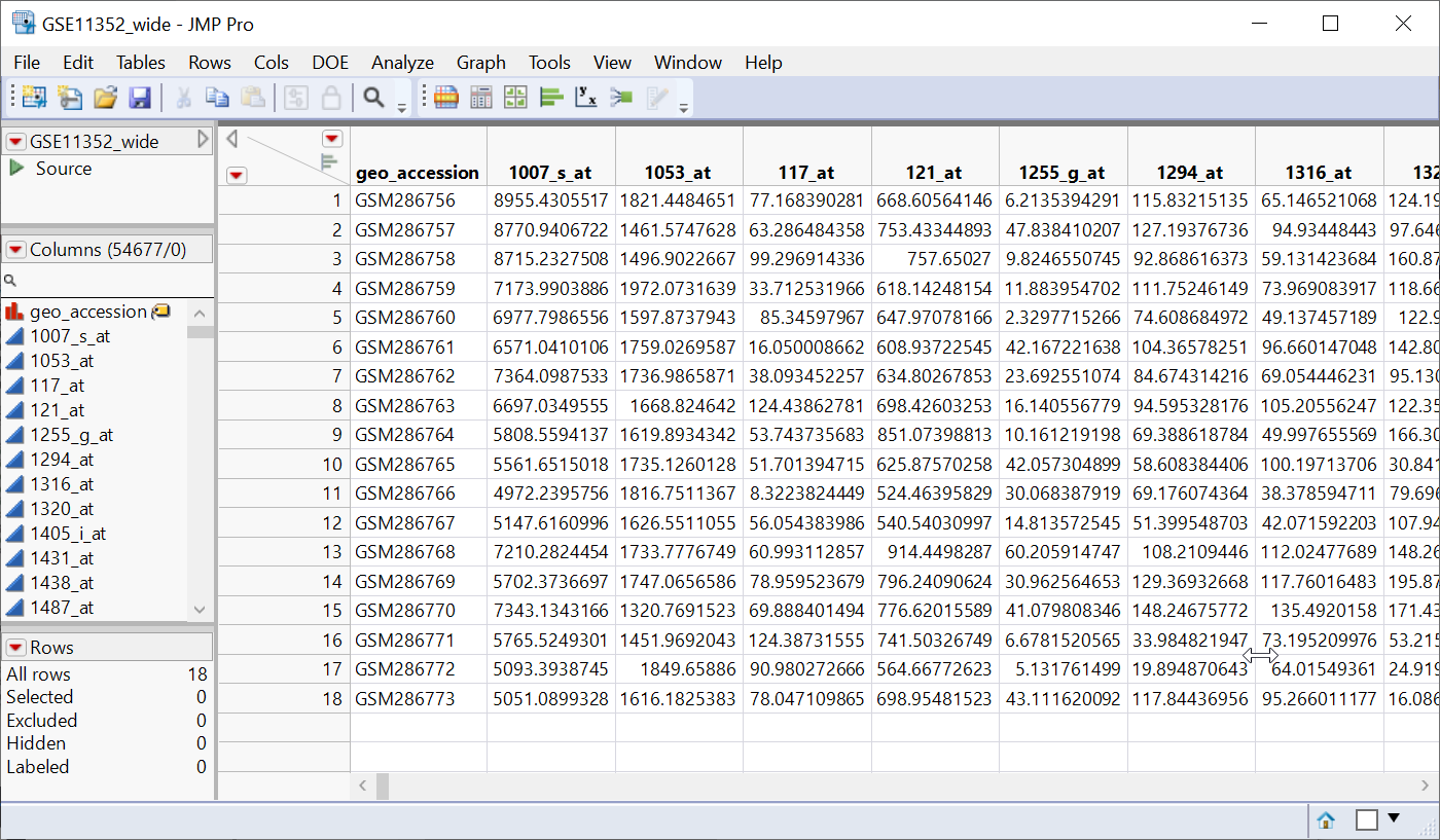
Note that the samples are now in rows and the genes assayed are in columns. This is now a wide data set.

Adding Experimental Design Information to the Data Table

One last thing is needed before we can proceed to analysis of the data. We must add the experimental design information to the data table. To do this we will join the GSE11352_series_matrix_samples.jmp table generated by the import process to the wide table be just created using JMP PRO's Join function.

Click on the GSE11352_series_matrix_samples.jmp table to make it active.

Select Tables > Join. The Join window opens.

Select the GSE11352_wide.jmp table as the table to join with.

Check the Merge same name columns box and specify geo_accession in both tables as the Match Columns.

The completed Join window appears as shown below.

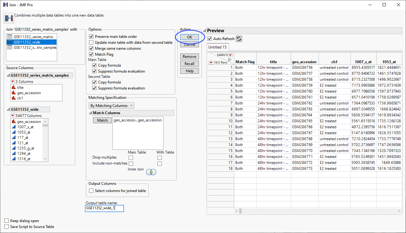
Click to generate the combined table.

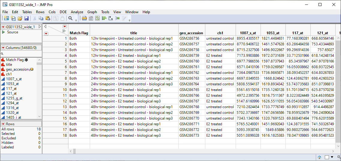
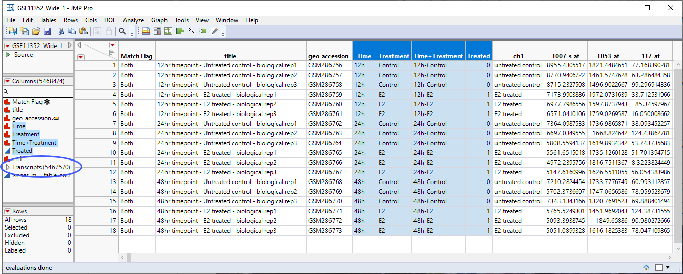
This table is almost ready for analysis. Several additional columns are needed. Use the Cols > New Column command to add separate columns for Time, Treatment, and Time+Treatment. Also, a column with numeric values of "1" and "0" indicating whether the sample was Treated or not, respectively. Finally, we will use the Cols > Group Columns command to group the data columns to make selecting them easier. The completed table is shown below.

Note: If you are planning to complete you analysis in one JMP session, you might want to consider temporarily linking the tables using JMP Pro's Virtual Join function instead of physically combining the data from the two tables into one. Virtually joining tables saves memory, because the same data are not replicated in every table that references them. However, the link is not maintained when you save the tables and exit JMP Pro, so if you plan to revisit oe extend your analysis at a later time, you should perform the normal join.

The final table is ready for analysis. See Analysis of Estradial-Responsive Genes in a Cell Line an example using this data.