Pharmacokinetics
The terms pharmacokinetics (PK) and pharmacodynamics (PD) are often described as “what the body does to the drug” and “what the drug does to the body”, respectively. PK/PD analyses are important for determining an appropriate dosing schedule to ensure that there is a sufficient quantity of the drug at the appropriate biological targets to observe beneficial activity. Ideally, this activity translates into an observable efficacy benefit in a clinical trial. On the safety side, PK/PD analyses are important to ensure that the drug does not reach concentrations that are likely to have negative effects which could translate into adverse events or other safety issues in a clinical trial. PK studies are often performed in healthy volunteers to guide dosing for subsequent clinical trials in patients (though particularly toxic drugs are always tested in patients). In these latter trials, a subset of patients may be selected for a PK sub-study to determine whether the PK behaves as expected, but it also serves as a means to acquire data on efficacy and safety endpoints which can then be described in conjunction with concentration data and associated PK parameters. Sometimes, particularly for topical medications, PK analyses are used to confirm that a drug is not detectable in blood, tissues, or other fluids to allay fears of greater systemic exposure beyond the treatment site. Finally, PK parameters are used to establish bioequivalence between branded products and their generic counterparts.
The JMP Fit Curve platform provides one- and two-compartment models for PK analysis using data available from the CDISC pharmacokinetics concentrations (PC) domain. Further, this report produces PK profiles that enable the user to view the data of each individual patient in the context of summary statistics derived across groups of patients.
Report Results Description
The standard Nicardipine sample study typically used in this User Guide does not have concentration data available in a PC domain and is suitable for use with this report. A simulated clinical trial data set, based on the Theophylline data that were described in Pinheiro & Bates (1995), is now included in the JMP Clinical Sample Data folder. Theophylline is a bronchodilator used to treat the symptoms of asthma and other lung diseases.
Running the Pharmacokinetics report for Theophylline using default settings generates the report shown below.
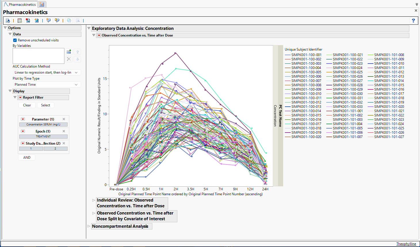
Output from the report is organized into sections. Each section contains one or more plots, data panels, data filters, or other elements that facilitate your analysis.
The Report contains the following elements:
Exploratory Data Analysis
Observed Concentration vs. Time after Dose
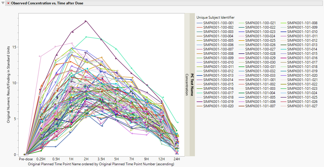
This plot displays observed concentrations for the Theophylline data by the planned time after dose for each patient in the trial.
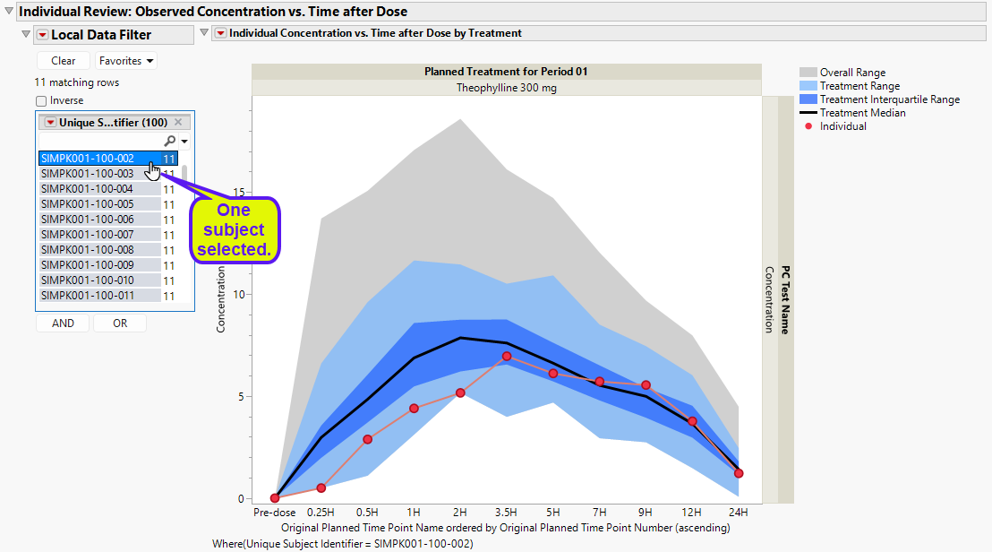
Individual Review - Observed Concentration vs Time after Dose
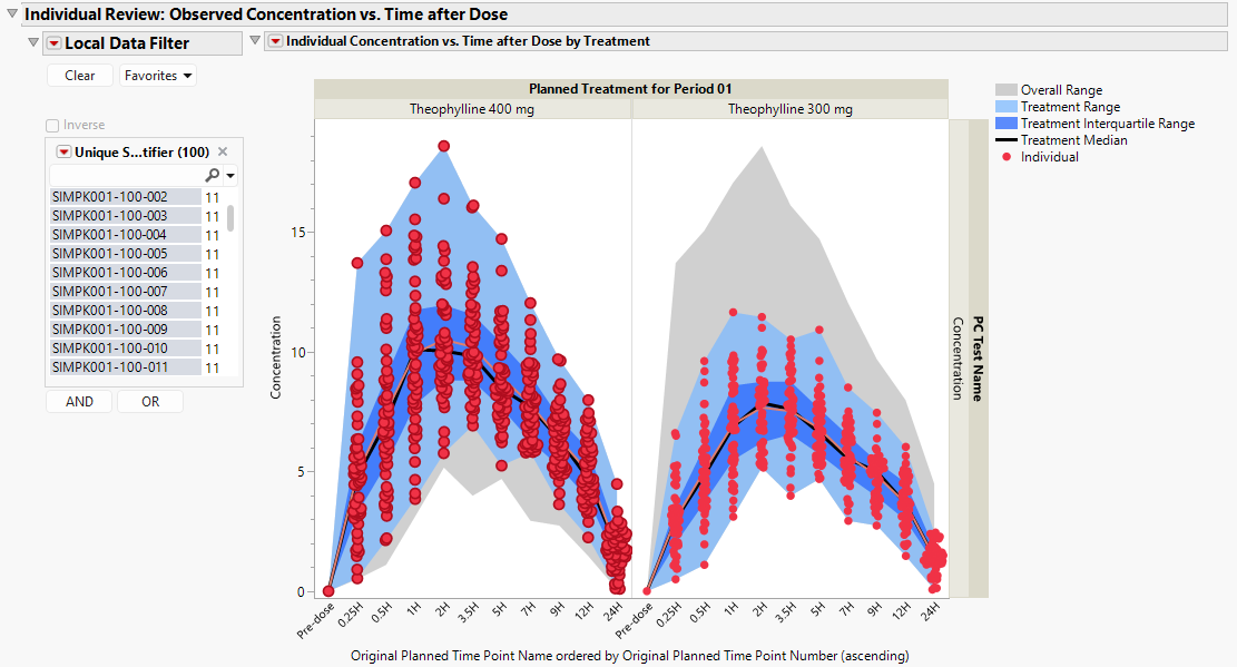
This plot displays concentration data by treatment for each patient (red dots), with shaded areas describing the overall range of concentration data (gray), the treatment-specific range of concentration data (light blue), and the treatment-specific interquartile range of concentration data (dark blue), along with the treatment-specific median concentration curve (black) and the individual concentration curve (red), which summarizes the mean concentration when more than one patient is presented.
The Local Data Filter can be used to subset to an individual patient to view their particular pk concentration profile. This view makes it possible to assess the individual’s pharmacokinetics in the context of the entire treatment arm as well as across all patients.
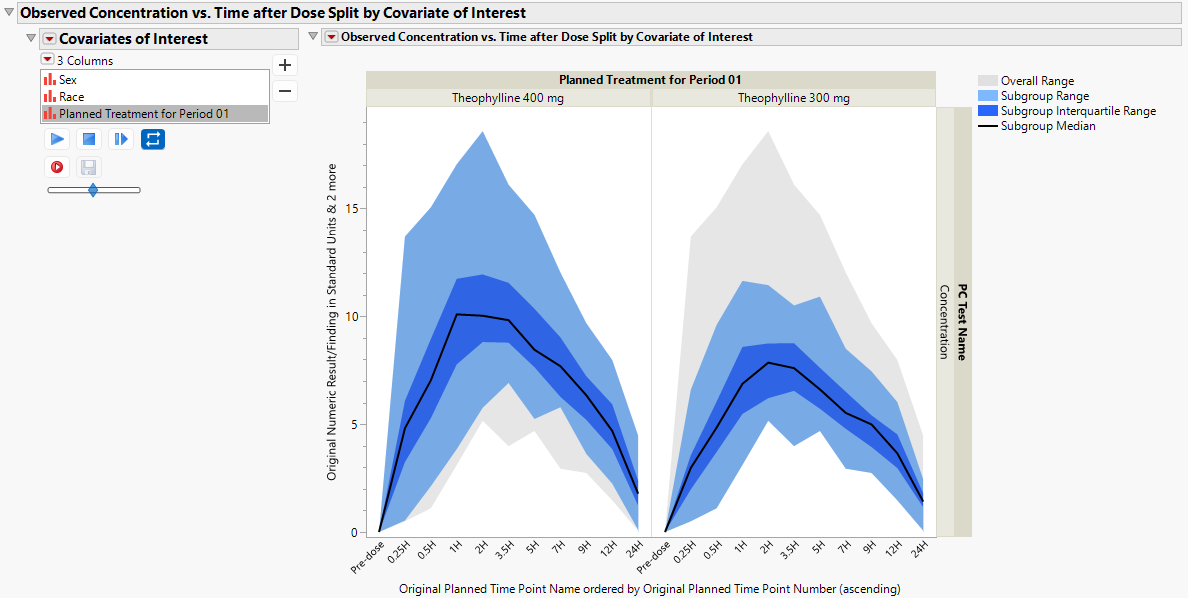
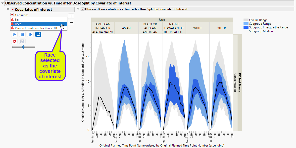
Observed Concentration vs. Time after Dose Split by Covariate of Interest
Concentration data can be further summarized by treatment group (default). In the figure below, the subgroup-specific range of concentration data (light blue), and the subgroup-specific interquartile range of concentration data (dark blue) are presented, along with the subgroup-specific median concentration curve (black).
Concentration data can be further summarized and presented by demographic subgroups, such as race.
Noncompartmental Analysis
Non-compartmental analysis (NCA), like non-parametric statistical analyses, applies a minimal number of assumptions to the underlying PK model. For a given patient, their concentration data are plotted across time and estimates of PK parameters are derived.
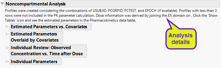
There are numerous plots (shown below) to assess the computed parameters of the non-compartmental analysis.
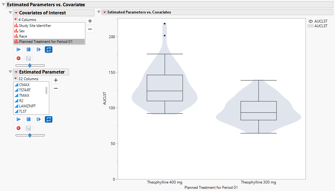
Estimated Parameters vs. Covariates
The box-plot with an overlaid violin plot shows the distribution of observed parameters by key covariates.
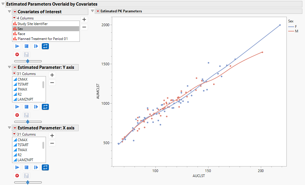
Estimated Parameters Overlaid by Covariates
The scatter plot enables you to view pairs of PK parameters with non-parametric curves to assess their bivariate relationship.
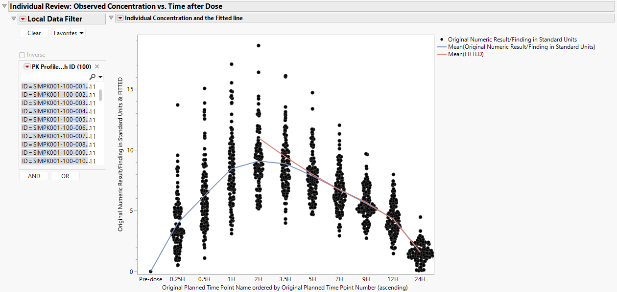
Individual Review: Observed Concentrations s. Time after Dose
The plot below presents concentrations with a curve fitted to the mean concentration at each time point (blue) and a curve fitted to the mean predicted concentration based on a linear fit over the elimination phase of the curve (red).
Individual Parameters
The following label lists computed parameters for each patient.
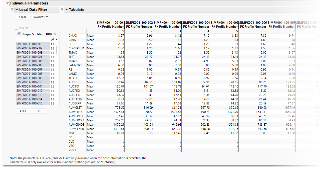
Computed parameters include the following:
| 1. | CMax (CMAX): The maximum observed concentration for a patient. |
| 2. | CMin (CMIN): The minimum observed non-zero concentration for a patient. |
| 3. | CLast (CLST): The last measurable concentration for a patient. |
| 4. | ĈLast (PREDCN): The last measurable predicted concentration for a patient. This is observable when subset to an individual patient. |
| 5. | TMax (TMAX): The time of the maximum observed concentration for a patient. |
| 6. | TLast (TLST): The time of the last measurable concentration for a patient. |
| 7. | TStart (TSTART): Observed time where the “start of regression” occurs. This is observable when subset to an individual patient. |
| 8. | λZN (LAMZNPT): The number of points included in the regression of the elimination constant. This is observable when subset to an individual patient. |
| 9. | R2 (RSQUARE): The maximum R2 from the best fitting regression line to determine the elimination constant. |
| 10. | λZ (LAMZ): the elimination constant, which is the rate at which a drug is eliminated from the body. |
| 11. | T1⁄2 (THALF): the half-life, which is the time required for the drug concentration to decrease by half. |
| 12. | AUCLast(AUCLST): The area under the curve, computed from time 0 to TLast, the last observable time point, which represents the total drug exposure in the body over time. |
| 13. | AUC∞ (AUCIFO): The area under the curve, computed from time 0 to ∞. |
| 14. | AUCPEO: The percentage of AUC∞ which is extrapolated i.e., (AUC∞-AUCLast)/AUC∞ × 100. |
| 15. | AUCPCX2: The percent of AUC∞ which is extrapolated relative to AUCLast, i.e., (AUC∞-AUCLast)/AUCLast × 100. |
| 16. | AUC(Last, ∞) (AUCEXOB): extrapolated AUC, from time TLast to ∞. |
| 17. | AUC(Last, ∞) (AUCEXPR): predicted extrapolated AUC, from time TLast to ∞. |
| 18. | AUMCLast (AUMCLST): The area under the first moment curve, from time 0 to TLast, the last observable time point. |
| 19. | AUMC∞ (AUMCIFO): The area under the first moment curve, computed from time 0 to ∞. |
| 20. | AUMCPEO: The percent of AUMC∞ which is extrapolated, i.e., (AUMC∞-AUMCLast)/AUMC∞ × 100. |
| 21. | AUMCPCX2: The percent of AUMC∞ which is extrapolated relative to AUMCLast , i.e., (AUMC∞-AUMCLast)/AUMCLast × 100. |
| 22. | AUMC(Last, ∞) (AUMCEXOB): extrapolated AUMC, from time TLast to ∞. |
| 23. | AUMC(Last, ∞) (AUMCEXPR): predicted extrapolated AUMC, from time TLast to ∞. |
| 24. | Mean Residence Time (MRT): represents the average time a drug molecule spends in the body. |
| 25. | Parameters that are available if drug exposure is available from an EX domain |
a. C0 (C0): the initial or extrapolated concentration at time 0 following an
intravenous bolus injection.
b. Plasma Clearance (CLO): the volume of blood or plasma cleared of a drug per
unit of time.
c. Volume of Distribution (VZO): the apparent volume of body fluid into which a
drug is distributed.
d. Volume Steady State (VSSO): the apparent volume of body fluid into which a
drug is distributed at steady state, which is the time at which the rate of drug
administration and elimination are equal.
Options
Data
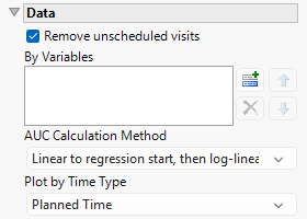
Remove unscheduled visits
You might or might not want to include unscheduled visits when you are analyzing findings by visit. Check the Remove unscheduled visits to exclude unscheduled visits.
By Variables
You can subdivide the subjects and run analyses for distinct groups by specifying one or more By Variables.
AUC Calculation Method
Use this widget to specify the method used to calculate the area under the curve (AUC). Options include Linear to regression start, then log-linear, Linear for the whole curve, Linear ascending, log-linear descending, and Log-linear for the whole curve, See AUC Calculation Method for more details.
Plot by Time Type
Use this widget to select the time measure, either planned time or actual time, to use in the plots.
Display
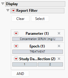
Report Filter
This widget enables you to subset and view subjects based on demographic characteristics and other criteria. By default, the filter in this report enables you to filter by parameter, Epoch, and Study Day of Collection. Refer to Data Filter for more information on filters.
General and Drill Down Buttons
Action buttons provide you with an easy way to drill down into your data. The following action buttons are generated by this report:
| • | Click  to reset all report options to default settings. to reset all report options to default settings. |
| • | Click  to view the associated data tables. Refer to Show Tables for more information. to view the associated data tables. Refer to Show Tables for more information. |
| • | Click  to generate a standardized pdf- or rtf-formatted report containing the plots and charts of selected sections. to generate a standardized pdf- or rtf-formatted report containing the plots and charts of selected sections. |
| • | Click  to generate a JMP Live report. Refer to Create Live Report for more information. to generate a JMP Live report. Refer to Create Live Report for more information. |
| • | Click  to take notes, and store them in a central location. Refer to Add Notes for more information. to take notes, and store them in a central location. Refer to Add Notes for more information. |
| • | Click  to read user-generated notes. Refer to View Notes for more information. to read user-generated notes. Refer to View Notes for more information. |
| • | Select one or more subjects, then click  to apply the Review Subject Filter and filter all reports in the review builder on the selected subjects. to apply the Review Subject Filter and filter all reports in the review builder on the selected subjects. |
| • | Select a group of subjects and click  to specify Derived Population Flags that enable you to distinguish the selected group of subjects from the general population based on their meeting specific criteria. to specify Derived Population Flags that enable you to distinguish the selected group of subjects from the general population based on their meeting specific criteria. |
Default Settings
Refer to Set Study Preferences for default Subject Level settings.
References
Pinheiro JC & Bates DM. (1995). Approximations to the Log-Likelihood Function in the Nonlinear Mixed-Effects Model. Journal of Computational and Graphical Statistics 4: 12–35.