Findings Forest
The Findings Forest report makes it straightforward to produce forest plots that summarize continuous and binary endpoints across treatments, visits, and, when available, time points. The goal is to provide summary statistics over time, enabling improved insight into endpoints compared with the often lengthy summary statistics tables that are provided in clinical reports, such as Table 1.
| Statistic | Nicardipine | Placebo | ||
|---|---|---|---|---|
| Baseline | n | Observed | XX | XX |
| Mean (SD) | XX.X (XX.XX) | XX.X (XX.XX) | ||
| Median | XX | XX | ||
| Min, Max | XX, XX | XX, XX | ||
| Visit 1 | n | Observed | XX | XX |
| Mean (SD) | XX.X (XX.XX) | XX.X (XX.XX) | ||
| Median | XX | XX | ||
| Min, Max | XX, XX | XX, XX | ||
| n | Change from Baseline | XX | XX | |
| Mean (SD) | XX.X (XX.XX) | XX.X (XX.XX) | ||
| Median | XX | XX | ||
| Min, Max | XX, XX | XX, XX | ||
| Visit 2 | n | Observed | XX | XX |
| … | … | … | … |

Methodology
Findings Forests analyzes each parameter individually, first determining whether the parameter is continuous or binary to apply the appropriate confidence interval. Binary variables have two levels, typically coded as 0 or 1; all other endpoints are considered continuous.
Binary
| • | 95% confidence intervals (CI) for proportions are calculated using the normal approximation, i.e.,  . |
| • | If at least one binary variable is identified, the report output includes a section titled Binary Variables, presented below Continuous Variables if at least one continuous variable is available. |
| • | Double forest plots present proportions by treatment, visit, and, when available, time point in the left panel. The right panel presents corresponding proportions for the subset of patients who were not in response at baseline (that is, those with a value of 0). For key primary and secondary endpoints, inclusion criteria might require patients to be non-responders at baseline, making these panels redundant (though mistakes often occur in practice). Less critical binary outcomes might include a mixture of positive and negative responses at baseline. |
Continuous
| • | 95% CIs for means are calculated using the t-distribution, i.e.,  . |
| • | If at least one continuous variable is identified, the report output includes a section titled Continuous Variables, presented below Binary Variables if at least one binary variable is available. |
| • | Double forest plots present means of the observed values by treatment, visit, and, when available, time point in the left panel. The right panel presents the means of change-from-baseline values. |
Time Points
The presence of time points is determined at the domain level. Six options are available for sorting and arranging the axes to organize content within the rows of the double forest plot (see Sort).
In practice, however, time points are often applied to only a subset of variables within a domain. For parameters to which time points do not apply (that is, all time point values are missing), the time point is excluded from the y-axis of the double forest plot. For parameters with a mixture of values attributed to specific time points and time point-agnostic values (that is, where the time point is missing), the missing time point value is listed as “NA”.
There might be a tendency for confidence intervals along the right axis to become slightly misaligned due to the length of the plot and the wrapping of text along the left axes. Minor adjustments to the size of the forest plot typically correct this misalignment.
Usage and Interpretation
Note: Click on the figures below to enlarge.
Example 1: Vital Signs Sorted by Visit, then Treatment
| Option Type | Option | Setting | |
|---|---|---|---|
| Data | Domain | VS (Vital Signs) | 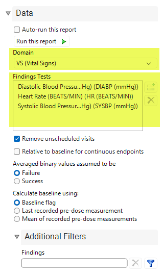
|
| Findings Tests | Diastolic Blood Pressure (mmHg)
(DIABP (mmHg) |
||
|
Heart Rate (BEATS/MIN) HR (BEATS/MIN) |
|||
|
Systolic Blood Pressure (mmHg) SYSBP (mmHg) |
|||
| All other options set to the default. | |||
Figure 1: Findings Forest Results for Nicardipine
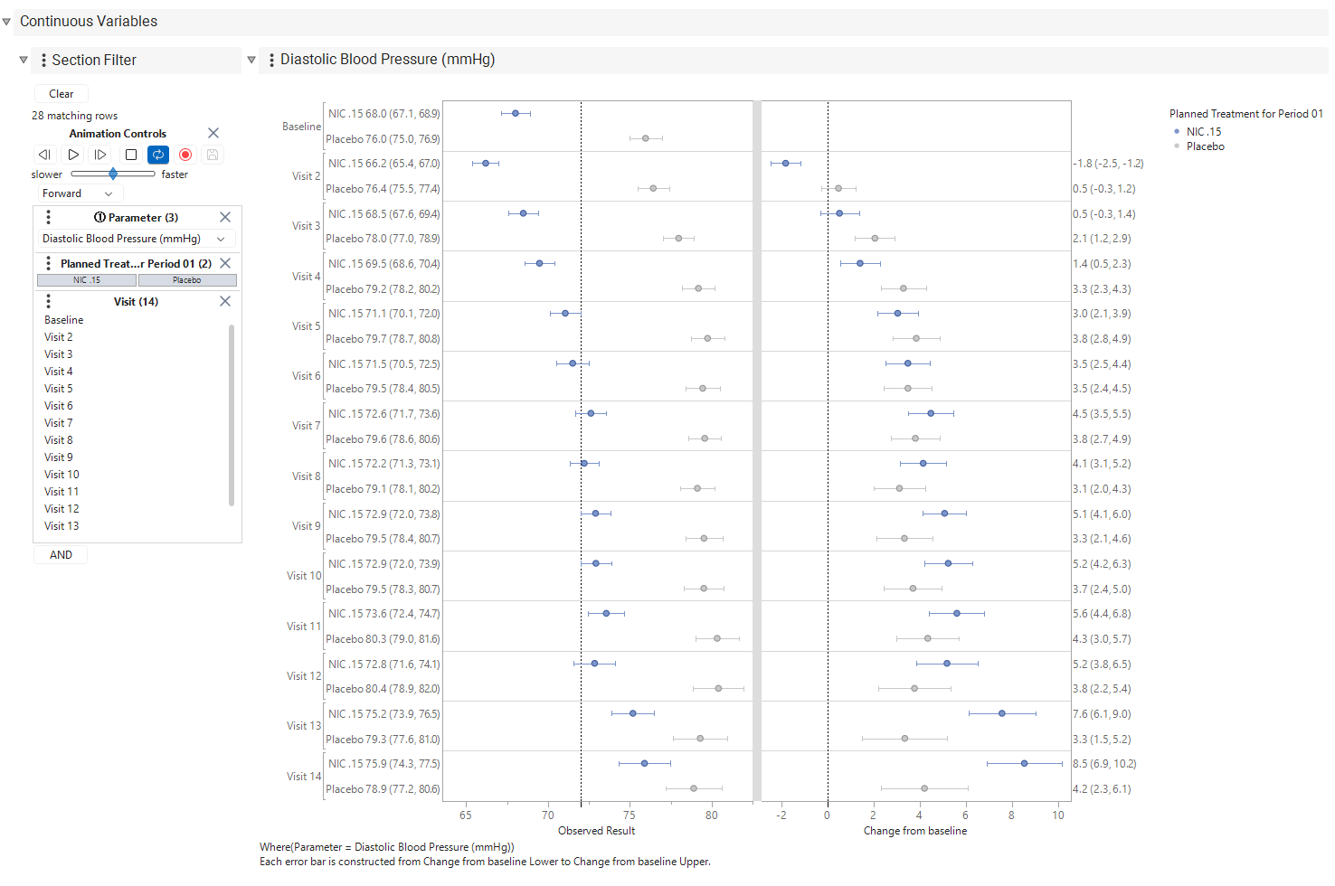
Figure 1 presents a double forest plot for diastolic blood pressure (DBP). In the left-hand panel, the mean and 95% CIs for observed DBP values are summarized by treatment arm and visit. In the right-hand panel, the mean and 95% CIs for change from baseline (CFB) are presented. There appears to be a difference between the treatment arms at baseline, with placebo patients exhibiting consistently higher mean DBP values over time. In the right-hand panel, except for Visit 2 for Nicardipine patients, the mean CFB for DBP increases over time in both treatment arms, with the difference widening across visits. By default, confidence interval text and reference lines for both observed values and change-from-baseline values are presented.
A note about how Findings Forests summarizes data prior to summarizing results by treatment, visit, and, when available, time point, observed values are first averaged within patient to ensure that each patient contributes at most one value to the computed summary statistics. This situation can occur when a second test is performed to confirm an unusual finding. For continuous variables, this approach is generally not problematic. However, for binary outcomes, this can result in values between 0 and 1. The Averaged binary values assumed to be option describes how instances in which a mixture of failures (0) and successes (1) are averaged should be handled. Note that an averaged value of 0 is always considered a failure, whereas an averaged value of 1 is always considered a success.
Example 2: Vital Signs Sorted by Treatment, then Visit
Figure 2 presents the double forest from Figure 1, sorted by treatment and visit. This arrangement makes it easier to observe how each treatment behaves over time, whereas Figure 1 makes it easier to compare treatments within each visit. The Section Filter can also be used to subset the data to key areas of interest.
Figure 2: Findings Forest Sorted by Treatment, Visit
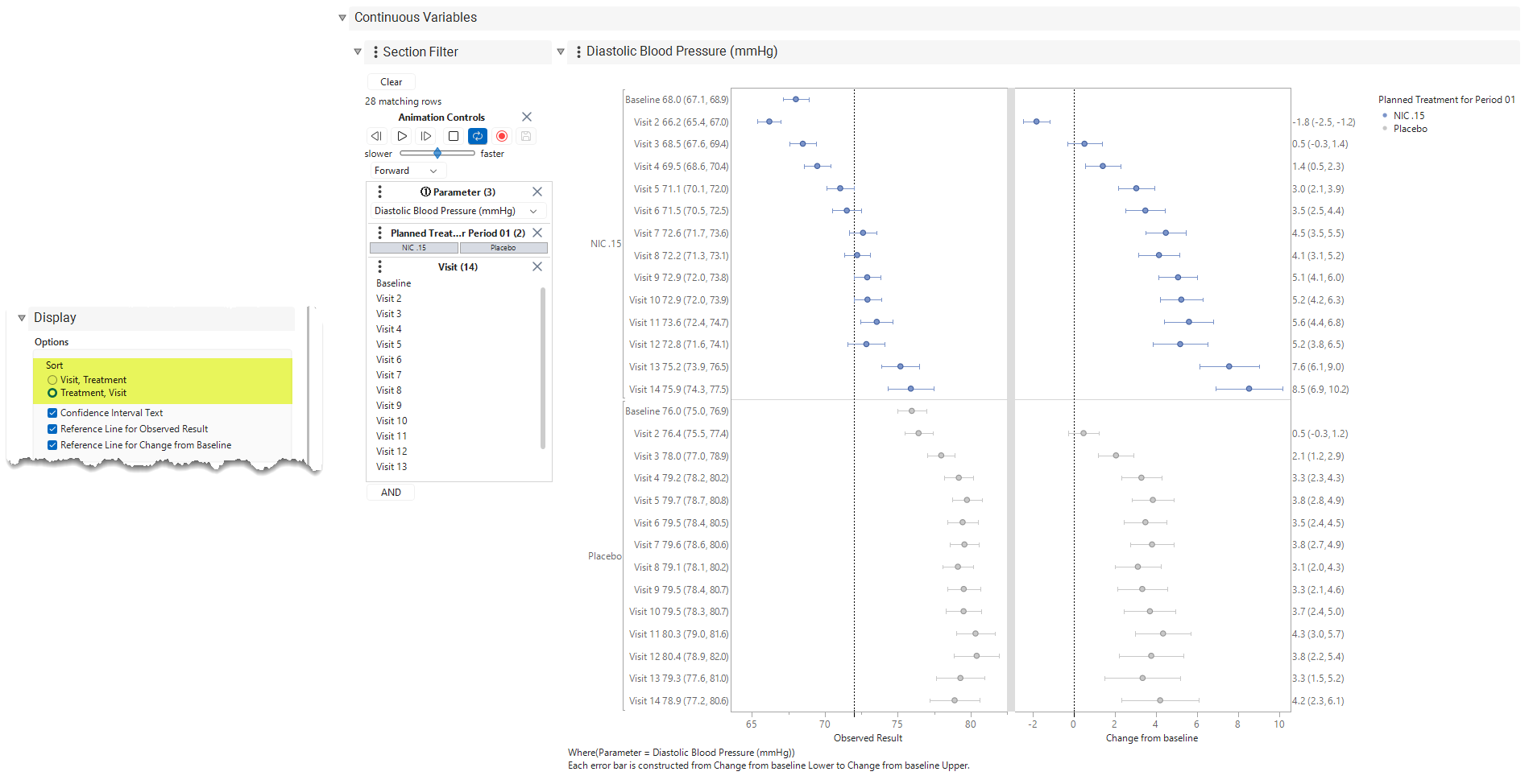
Figure 2 presents a double forest plot for diastolic blood pressure (DBP). In the left-hand panel, the mean and 95% CIs for observed DBP values are summarized by treatment arm and visit. In the right-hand panel, the mean and 95% CIs for change from baseline (CFB) are presented. There appears to be a difference between the treatment arms at baseline, with placebo patients exhibiting consistently higher mean DBP values over time. In the right-hand panel, except for Visit 2 for Nicardipine patients, the mean CFB for DBP increases over time in both treatment arms, with the difference widening across visits.
By default, confidence interval text and reference lines for both observed values and change-from-baseline values are presented, though Display options make it possible to modify these choices.
Options
Data
Domain
 View/Hide Details.
Use this widget to select a specific study Domain.
Findings Tests
View/Hide Details.
Use this widget to select specific Findings tests. If you leave this field blank, all tests are run.
| 8 | Click  to open the Add window (shown below) that lists available test names (shown below). |
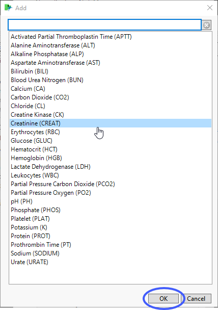
| 8 | Select the desired test(s) and click to add them to the text box. |
Remove unscheduled visits
View/Hide Details.
You might want to include unscheduled visits when you are analyzing findings by visit.
By default, this box is checked. When it is checked, records are excluded from the analysis if the VISIT variable exists and contains the text "unscheduled" for those records. If the box is not checked, all records are included regardless of the VISIT status.
For some reports, you might have to specify Visits as the Time Scale to enable this field.
Relative to baseline for continuous endpoints
View/Hide Details.
Checking this option modifies the double forest plots for continuous endpoints to present means of percent of baseline in the left hand panel and means of percent change from baseline in the right hand panel.
Averaged binary values assumed to be
View/Hide Details.
Use this option to specify how to represent instances when a mixture of failures (0) and successes (1) are averaged. Note that an averaged value of 0 is always considered a failure, while an averaged value of 1 is always considered a success. When a mixture of failures and success are averaged results in a value that is not 0 or 1, assumptions are made according to the following options.
| • | Choosing Failure assumes that a mixture of successes and failures is considered a failure. This approach is more conservative for endpoints where success is considered a positive outcome and is less conservative for endpoints where success is considered a negative outcome. It is likely more appropriate to make this assumption for efficacy endpoints to ensure a robust response. |
| • | Choosing Success assumes that a mixture of successes and failures is considered a success. This approach is more conservative for endpoints where success is considered a negative outcome and is less conservative for endpoints where success is considered a positive outcome. It is likely more appropriate to make this assumption for safety endpoints to capture any instance of a negative outcome. |
Calculate baseline as:
View/Hide Details.
Use this widget to use the flagged baseline record, last recorded pre-dose measurement, or the mean of all the measurements taken during the baseline time window as the baseline measurement.
By default, the flagged baseline record is used.
The following test measurements are considered when forming the baseline measurement:
| • | Those flagged as baseline |
| • | Those taken prior to Study Day 1 |
Choose Last recorded pre-dose measurement to use the last recorded predose test measurement (out of the test measurement pool generated from the above list) as the baseline measurement.
Choose Mean of recorded pre-dose measurements to average these predose test measurements to form the baseline measurement.
Note: When the selected option to calculate baseline is to use the baseline flag and there are two records flagged as baseline, JMP Clinical uses the last record. This differs from JMP Clinical version 8.1, where the mean of the flagged baseline values was used.
Additional Filters - Findings
View/Hide Details
This filter lets you restrict your analysis to only those subjects that meet specific criteria at the level of the specified Findings domain (EG, LB, or VS) .

This filters uses JMP WHERE clauses to Select Rows that meet the specified criteria. To use this filter, you must enter the JSL (JMP Scripting Language) expressions that constitute the WHERE clause in the appropriate text box for specific filtering of findings. Note: This is an advanced concept that not only requires some basic knowledge of the JSL WHERE clause syntax (similar to, but different from, SQL), but also an understanding of the exact variables in the tables in the study.
Risk indicators are calculated using this subset only.
To specify a Findings filter:
| 8 | Click  to open the WHERE Clause Builder to construct the desired filter. |
| 8 | Click  to clear the filter. |
Note: To filter subjects with a specific event or finding, one could also use the Subpopulation Builder on any domain of interest. For example, filter to all subjects that exhibit cardiac failure ( :Customized Query 01 Name == "Cardiac failure" ) and run all reports on those.
Display
Sort
View/Hide Details.
Use this option to specify how you want to view records of interest.
When time points are present, six sorting methods are offered for you to choose.
| • | Visit, Timepoint, Treatment - Choose to sort and present first by Visit, then by Time point, and finally by Treatment. |
| • | Visit, Treatment, Timepoint - Choose to sort and present first by Visit, then by Treatment, and finally by Time point. |
| • | Treatment, Visit, Timepoint - Choose to sort and present first by Treatment, then by Visit, and finally by Time point. |
| • | Treatment, Timepoint, Visit - Choose to sort and present first by Treatment, then by Time point, and finally by Visit. |
| • | Timepoint, Treatment, Visit - Choose to sort and present first by Time point, then by Treatment, and finally, by Visit. |
| • | Timepoint, Visit, Treatment - Choose to sort and present first by Time point, then by Visit, and finally by Treatment. |
In the case where time points are not present, there are two choices:
| • | Visit, Treatment (default): Choose to sort and present first by Visit, then by Treatment. |
| • | Treatment, Visit: Choose to sort and present first by Treatment, then by Visit. |
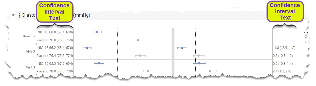
Confidence Interval Text
View/Hide Details.
Check this option to specify whether the confidence interval text should be displayed in the double forest plots.
This text is formatted as: Mean (Upper Limit, Lower Limit) and is displayed to either side of the double forest plot. as shown below:
Reference Line for Observed Result
View/Hide Details.
Check this option to add reference lines to the left panels for both continuous and binary variables.
The reference line is based on the average observed result at baseline for all patients, which makes it easier to observe changes over time relative to the overall mean at baseline. Note that a similar reference line is never added to the right panel for binary variables since this would always be 0 since patients are subset to non-responders.
Reference Line for Change from Baseline
View/Hide Details.
Check this option to add reference lines to the right panels for both continuous variables. This reference line is 0, making it easier to observe changes over time relative to baseline.
Action Buttons
Action buttons an easy way for you to drill down into your data. The following action buttons are generated by this report:
Click here to display the list and description of the Report Action buttons..
| • | Click  to rerun the report using default settings. |
| • | Click  to view the associated data tables. Refer to Show Tables for more information. |
| • | Click  to generate a standardized PDF- or RTF-formatted report containing the plots and charts of selected sections. |
| • | Click  to generate a JMP Live report. Refer to Create Live Report for more information. |
| • | Click  to take notes, and store them in a central location. Refer to Add Notes for more information. |
| • | Click  to read user-generated notes. Refer to View Notes for more information. |
Default Settings
Refer to Set Study Preferences for default Subject Level settings.